As time-series data becomes ubiquitous, measuring change is vital to understanding the world. Here at Timescale, we use our PostgreSQL and TimescaleDB superpowers to generate insights into the data to see what and how things changed and when they changed—that’s the beauty of time-series data. But, if you have data showing past and present trends, can you predict the future? Cue in time-series forecasting.

In the simplest terms, time-series forecasting is a technique that utilizes historical and current data to predict future values over a period of time or a specific point in the future. By analyzing data that we stored in the past, we can make informed decisions that can guide our business strategy and help us understand future trends.

Some of you may be asking yourselves what the difference is between time-series forecasting and algorithmic predictions using, for example, machine learning. Well, machine-learning techniques such as random forest, gradient boosting regressor, and time delay neural networks can help extrapolate temporal data, but they are far from the only available options or the best ones (as you will see in this article). The most important property of a time-series algorithm is the ability to extrapolate patterns outside of the domain of training data, which most machine-learning techniques cannot do by default. This is where specialized time-series forecasting techniques come in.

There are plenty of forecasting techniques to choose from; this article will help you understand the most popular ones. From simple linear regression models to complex and vast neural networks, each forecasting method has its own benefits and drawbacks.

Let’s check them out.

Applications of Time-Series Forecasting

Many industries and scientific fields utilize time-series forecasting. Examples:

• Business planning
• Control engineering
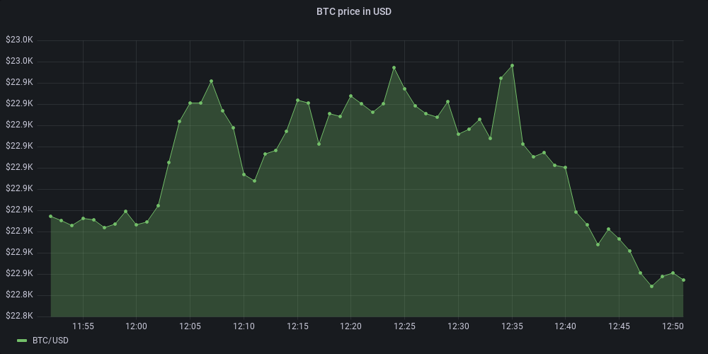
• Cryptocurrency trends
• Financial markets
• Modeling disease spreading
• Pattern recognition
• Resources allocation
• Signal processing
• Sports analytics
• Statistics
• Weather forecasting

The list is already quite long, but anyone with access to accurate historical data can utilize time-series analysis methods to forecast future developments and trends.

When Is Time-Series Forecasting Useful?

Even though time-series forecasting may seem like a universally applicable technique, developers need to be aware of some limitations. Because forecasting isn’t a strictly defined method but rather a combination of data analysis techniques, analysts and data scientists must consider the limitations of the prediction models and the data itself.

The most crucial step when considering time-series forecasting is understanding your data model and knowing which business questions need to be answered using this data. By diving into the problem domain, a developer can more easily distinguish random fluctuations from stable and constant trends in historical data. This is useful when tuning the prediction model to generate the best forecasts and even considering the method to use.

When using time-series analysis, you must consider some data limitations. Common problems include generalizing from a single data source, obtaining appropriate measurements, and accurately identifying the correct model to represent the data.

What to Consider When You Do Time-Series Forecasting

There are quite a few factors associated with time-series forecasting, but the most important ones include the following:

• Amount of data
• Data quality
• Seasonality
• Trends
• Unexpected events

The amount of data is probably the most important factor (assuming that the data is accurate). A good rule of thumb would be the more data we have, the better our model will generate forecasts. More data also makes it much easier for our model to distinguish between trends and noise in the data.

Data quality entails some basic requirements, such as having no duplicates, a standardized data format, and collecting data consistently or at regular intervals.

Seasonality means that there are distinct periods when the data contains consistent irregularities. For example, if an online web shop analyzed its sales history, it would be evident that the holiday season results in increased sales. In this example, we can deduce the correlation intuitively, but there are many other examples where analysis methods such as time-series forecasting are needed to detect such consumer behavior.

Trends are probably the most essential information you are looking for. They indicate whether a variable in the time series will increase or decrease in a given period. We can also calculate the probability of a trend to make even more informed decisions with our data.

Unexpected events (sometimes called noise or irregularities) can always occur, and we need to consider that when creating a prediction model. They present noise in historical data, and they are also not predictable.

Overview of Time-Series Forecasting Methods

Below is a basic overview of several forecasting methods that we covered and the theory behind them:

• Time-series decomposition
• Time-series regression models
• Exponential smoothing
• ARIMA models
• Neural networks
• TBATS

Time-Series Decomposition

Time-series decomposition is a method for explicitly modeling the data as a combination of seasonal, trend, cycle, and remainder components instead of modeling it with temporal dependencies and autocorrelations. It can either be performed as a standalone method for time-series forecasting or as the first step in better understanding your data.

When using a decomposition model, you need to forecast future values for each component above and then sum these predictions to find the most accurate overall forecast. The most relevant decomposition forecasting techniques using decomposition are Seasonal-Trend decomposition using LOESS, Bayesian structural time series (BSTS), and Facebook Prophet.

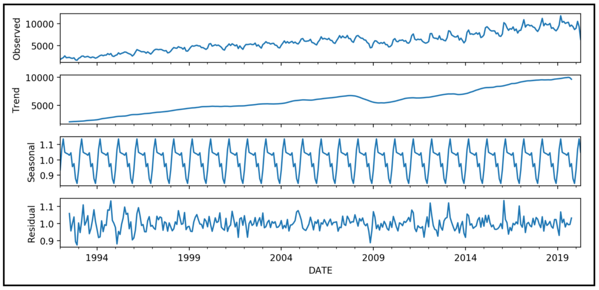
Decomposition based on rates of change

Decomposition based on rates of change is a technique for analyzing seasonal adjustments. This technique constructs several component series, which combine (using additions and multiplications) to make the original time series. Each of the components has a specific characteristic or type of behavior. They usually include:

• T_t: The trend component at time t describes the long-term progression of the time series. A trend is present when there is a consistent increase or decrease in the direction of the data. The trend component isn’t constrained to a linear function.
• C_t: The cyclical component at time t reflects repeated but non-periodic fluctuations. The duration of these fluctuations depends on the nature of the time series.
• S_t: The seasonal component at time t reflects seasonality (seasonal variation). You find seasonal patterns in time series that are influenced by seasonal factors. Seasonality usually occurs in a fixed and known period (for example, holiday seasons).
• I_t: The irregular component (or "noise") at time t represents random and irregular influences. It is the remainder of the time series after removing other components.
  

Additive decomposition: Additive decomposition implies that time-series data is a function of the sum of its components. This can be represented with the following equation:

y_t = T_t + C_t + S_t + I_t

where y_t is the time-series data, T_t is the trend component, C_t is the cycle component, S_t is the seasonal component, and I_t is the remainder.

Multiplicative decomposition: Instead of using addition to combine the components, multiplicative decomposition defines temporal data as a function of the product of its components. In the form of an equation:

y_t = T_t * C_t * S_t * I_t

The question is how to identify a time series as additive or multiplicative. The answer is in its variation. If the magnitude of the seasonal component is dynamic and changes over time, it’s safe to assume that the series is multiplicative. If the seasonal component is constant, the series is additive.

Some methods combine the trend and cycle components into one trend-cycle component. It can be referred to as the trend component even when it contains visible cycle properties. For example, when using seasonal-trend decomposition with LOESS, the time series is decomposed into seasonal, trend, and irregular (also called noise) components, where the cycle component is included in the trend component.

Time-Series Regression Models

Time-series regression is a statistical method for forecasting future values based on historical data. The forecast variable is also called the regressand, dependent, or explained variable. The predictor variables are sometimes called the regressors, independent, or explanatory variables. Regression algorithms attempt to calculate the line of best fit for a given dataset. For example, a linear regression algorithm could try to minimize the sum of the squares of the differences between the observed value and predicted value to find the best fit.

Let’s look at one of the simplest regression models, simple linear regression. The regression model describes a linear relationship between the forecast variable y and a simple predictor variable x:

y_t = β₀ + β₁ * x_t + ε_t

The coefficients β₀ and β₁ denote the line's intercept and slope. The slope β₁ represents the average predicted change in y resulting from a one-unit increase in x:

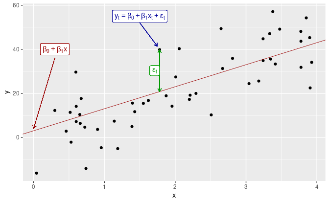
It’s important to note that the observations aren’t perfectly aligned on the straight line but are somewhat scattered around it. Each of the observations y_t is made up of a systematic component of the model (β₀ + β₁ * x_t ) and an “error” component (ε_t). The error component doesn’t have to be an actual error; the term encompasses any deviations from the straight-line model.

As you can see, a linear model is very limited in approximating underlying functions, which is why other regression models, like Least squares estimation and Nonlinear regression, may be more useful.

Exponential Smoothing

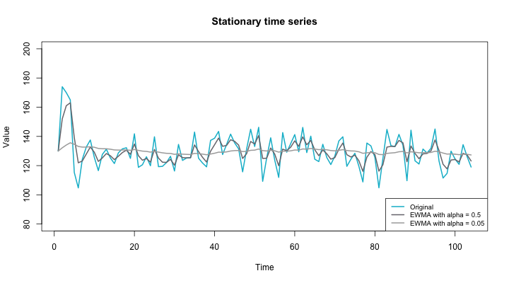
When it comes to time-series forecasting, data smoothing can tremendously improve the accuracy of our predictions by removing outliers from a time-series dataset. Smoothing leads to increased visibility of distinct and repeating patterns hidden between the noise.

Exponential smoothing is a rule-of-thumb technique for smoothing time-series data using the exponential window function. Whereas the simple moving average method weighs historical data equally to make predictions, exponential smoothing uses exponential functions to calculate decreasing weights over time. Different types of exponential smoothing include simple exponential smoothing and triple exponential smoothing (also known as the Holt-Winters method).

ARIMA Models

AutoRegressive Integrated Moving Average, or ARIMA, is a forecasting method that combines both an autoregressive model and a moving average model. Autoregression uses observations from previous time steps to predict future values using a regression equation. An autoregressive model utilizes a linear combination of past variable values to make forecasts:

An autoregressive model of order p can be written as:

y_t = c + ϕ₁y_t-1 + ϕ₂y_t−2 + ⋯ + ϕ_py_t−p + ε_t

where ε_t is white noise. This form is like a multiple regression model but with delayed values of y_t as predictors. We refer to this as an AR(p) model, an autoregressive model of order p.

On the other hand, a moving average model uses a linear combination of forecast errors for its predictions:

y_t = c + ε_t + θ₁ε_t−1 + θ₂ε_t−2 + ⋯ + θ_qε_t−q

where ε_t represents white noise. We refer to this as an MA(q) model, a moving average model of order q. The value of εt is not observed, so we can’t classify it as a regression in the usual sense.

If we combine differencing with autoregression and a moving average model, we obtain a non-seasonal ARIMA model. The complete model can be represented with the following equation:

y′_t = c + ϕ₁y′_t−1 + ⋯ + ϕ_py′_t−p + θ₁ε_t−1 + ⋯ + θ_qε_t−q + ε_t

where y′_t is the differenced series (find more on differencing here). The “predictors” on the right-hand side combine the lagged values y_t and lagged errors. The model is called an ARIMA( p, d, q) model. The model's parameters are:

• p: the order of the autoregressive component
• d: the degree of first differencing involved
• q: the order of the moving average part

The SARIMA model (Seasonal ARIMA) is an extension of the ARIMA model. This extension adds a linear combination of seasonal past values and forecast errors.

Neural Networks

Neural networks are also gaining traction regarding tasks such as classification and prediction. A neural network can sufficiently approximate any continuous functions for time-series forecasting. While classical methods like ARMA and ARIMA assume a linear relationship between inputs and outputs, neural networks are not bound by this constraint. They can approximate any nonlinear function without prior knowledge about the properties of the data series.

Neural networks such as multilayer perceptrons (MLPs) offer multiple advantages worth considering:

• Robust to noise: Neural networks are robust to noise when it comes to input data and robust in the mapping function. This robustness is useful when working with data that contains missing values.
• Nonlinear support: Neural networks are not bound to strong assumptions and a rigid mapping function. They can continuously learn from new linear and nonlinear relationships.
• Multivariate inputs: Multivariate forecasting is supported because the number of input features is entirely variable.
• Multi-step forecasts: The number of output values is variable as well.

TBATS

A lot of time series contain complex and multiple seasonal patterns (e.g., hourly data containing a daily pattern, weekly pattern, and annual pattern). The most popular models (e.g., ARIMA and exponential smoothing) can only account for one seasonality.

A TBATS model can deal with complex seasonalities (e.g., non-integer seasonality, non-nested seasonality, and large-period seasonality) with no seasonality constraints, making it possible to create detailed, long-term forecasts. But there is also a drawback to using TBATS models. They can be slow when calculating predictions, especially with long time series.

TBATS is an acronym for some of the most important features that the model offers:

• T: Trigonometric seasonality
• B: Box-Cox transformation
• A: ARIMA errors
• T: Trend
• S: Seasonal components

Conclusion

Time-series forecasting is a powerful method for predicting future trends and values in time-series data. Time-series forecasting holds tremendous value for your business development as it leverages historical data with a time component. While there are many forecasting methods to choose from, most of them are focused on specific situations and types of data, making it relatively easy to choose the right one.

If you are interested in time-series forecasting, look at this tutorial about analyzing Cryptocurrency market data. Using a time-series database like TimescaleDB, you can ditch complex analysis techniques that require a lot of custom code and instead use the SQL query language to generate insights.

Next steps

• Learn how you can do time-series forecasting using Python.
• See how this data scientist built a time-series forecasting pipeline using TimescaleDB.