

Point-in-Time PostgreSQL Database and Query Monitoring With pg_stat_statements
Database monitoring is a crucial part of effective data management and building high-performance applications. In our previous blog post, we discussed how to enable pg_stat_statements (and that it comes standard on all Timescale instances), what data it provides, and demonstrated a few queries that you can run to glean useful information from the metrics to help pinpoint problem queries.
We also discussed one of the few pitfalls with pg_stat_statements: all of the data it provides is cumulative since the last server restart (or a superuser reset the statistics).
While pg_stat_statements can work as a go-to source of information to determine where initial problems might be occurring when the server isn’t performing as expected, the cumulative data it provides can also pose a problem when said server is struggling to keep up with the load.
The data might show that a particular application query has been called frequently and read a lot of data from the disk to return results, but that only tells part of the story. With cumulative data, it's impossible to answer specific questions about the state of your cluster, such as:
- Does it usually struggle with resources at this time of day?
- Are there particular forms of the query that are slower than others?
- Is it a specific database that's consuming resources more than others right now?
- Is that normal given the current load?
The database monitoring information that pg_stat_statements provides is invaluable when you need it. However, it's most helpful when the data shows trends and patterns over time to visualize the true state of your database when problems arise.
It would be much more valuable if you could transform this static, cumulative data into time-series data, regularly storing snapshots of the metrics. Once the data is stored, we can use standard SQL to query delta values of each snapshot and metric to see how each database, user, and query performed interval by interval. That also makes it much easier to pinpoint when a problem started and what query or database appears to be contributing the most.
In this blog post (a sequel to our previous 101 on the subject), we'll discuss the basic process for storing and analyzing the pg_stat_statements snapshot data over time using TimescaleDB features to store, manage, and query the metric data efficiently.
Although you could automate the storing of snapshot data with the help of a few PostgreSQL extensions, only TimescaleDB provides everything you need, including automated job scheduling, data compression, data retention, and continuous aggregates to manage the entire solution efficiently.
PostgreSQL Database Monitoring 201: Preparing to Store Data Snapshots
Before we can query and store ongoing snapshot data from pg_stat_statements, we need to prepare a schema and, optionally, a separate database to keep all of the information we'll collect with each snapshot.
We're choosing to be very opinionated about how we store the snapshot metric data and, optionally, how to separate some information, like the query text itself. Use our example as a building block to store the information you find most useful in your environment. You may not want to keep some metric data (i.e., exec_stddev), and that's okay. Adjust based on your database monitoring needs.
Create a metrics database
Recall that pg_stat_statements tracks statistics for every database in your PostgreSQL cluster. Also, any user with the appropriate permissions can query all of the data while connected to any database. Therefore, while creating a separate database is an optional step, storing this data in a separate TimescaleDB database makes it easier to filter out the queries from the ongoing snapshot collection process.
We also show the creation of a separate schema called statements_history to store all of the tables and procedures used throughout the examples. This allows a clean separation of this data from anything else you may want to do within this database.
psql=> CREATE DATABASE statements_monitor;

psql=> \c statements_monitor;

psql=> CREATE EXTENSION IF NOT EXISTS timescaledb;

psql=> CREATE SCHEMA IF NOT EXISTS statements_history;
Create hypertables to store snapshot data
Whether you create a separate database or use an existing TimescaleDB database, we need to create the tables to store the snapshot information. For our example, we'll create three tables:
snapshots(hypertable): a cluster-wide aggregate snapshot of all metrics for easy cluster-level monitoringqueries: separate storage of query text byqueryid,rolname, anddatnamestatements(hypertable): statistics for each query every time the snapshot is taken, grouped byqueryid,rolname, anddatname
Both the snapshot and statements tables are converted to a hypertable in the following SQL. Because these tables will store lots of metric data over time, making them hypertables unlocks powerful features for managing the data with compression and data retention, as well as speeding up queries that focus on specific periods of time. Finally, take note that each table is assigned a different chunk_time_interval based on the amount and frequency of the data that is added to it.
The snapshots table, for instance, will only receive one row per snapshot, which allows the chunks to be created less frequently (every four weeks) without growing too large. In contrast, the statements table will potentially receive thousands of rows every time a snapshot is taken and so creating chunks more frequently (every week) allows us to compress this data more frequently and provides more fine-grained control over data retention.
The size and activity of your cluster, along with how often you run the job to take a snapshot of data, will influence what the right chunk_time_interval is for your system. More information about chunk sizes and best practices can be found in our documentation.
/*
 * The snapshots table holds the cluster-wide values
 * each time an overall snapshot is taken. There is
 * no database or user information stored. This allows
 * you to create cluster dashboards for very fast, high-level
 * information on the trending state of the cluster.
 */
CREATE TABLE IF NOT EXISTS statements_history.snapshots (
    created timestamp with time zone NOT NULL,
    calls bigint NOT NULL,
    total_plan_time double precision NOT NULL,
    total_exec_time double precision NOT NULL,
    rows bigint NOT NULL,
    shared_blks_hit bigint NOT NULL,
    shared_blks_read bigint NOT NULL,
    shared_blks_dirtied bigint NOT NULL,
    shared_blks_written bigint NOT NULL,
    local_blks_hit bigint NOT NULL,
    local_blks_read bigint NOT NULL,
    local_blks_dirtied bigint NOT NULL,
    local_blks_written bigint NOT NULL,
    temp_blks_read bigint NOT NULL,
    temp_blks_written bigint NOT NULL,
    blk_read_time double precision NOT NULL,
    blk_write_time double precision NOT NULL,
    wal_records bigint NOT NULL,
    wal_fpi bigint NOT NULL,
    wal_bytes numeric NOT NULL,
    wal_position bigint NOT NULL,
    stats_reset timestamp with time zone NOT NULL,
    PRIMARY KEY (created)
);

/*
 * Convert the snapshots table into a hypertable with a 4 week
 * chunk_time_interval. TimescaleDB will create a new chunk
 * every 4 weeks to store new data. By making this a hypertable we
 * can take advantage of other TimescaleDB features like native
 * compression, data retention, and continuous aggregates.
 */
SELECT * FROM create_hypertable(
    'statements_history.snapshots',
    'created',
    chunk_time_interval => interval '4 weeks'
);

COMMENT ON TABLE statements_history.snapshots IS
$$This table contains a full aggregate of the pg_stat_statements view
at the time of the snapshot. This allows for very fast queries that require a very high level overview$$;

/*
 * To reduce the storage requirement of saving query statistics
 * at a consistent interval, we store the query text in a separate
 * table and join it as necessary. The queryid is the identifier
 * for each query across tables.
 */
CREATE TABLE IF NOT EXISTS statements_history.queries (
    queryid bigint NOT NULL,
    rolname text,
    datname text,
    query text,
    PRIMARY KEY (queryid, datname, rolname)
);

COMMENT ON TABLE statements_history.queries IS
$$This table contains all query text, this allows us to not repeatably store the query text$$;


/*
 * Finally, we store the individual statistics for each queryid
 * each time we take a snapshot. This allows you to dig into a
 * specific interval of time and see the snapshot-by-snapshot view
 * of query performance and resource usage
*/
CREATE TABLE IF NOT EXISTS statements_history.statements (
    created timestamp with time zone NOT NULL,
    queryid bigint NOT NULL,
    plans bigint NOT NULL,
    total_plan_time double precision NOT NULL,
    calls bigint NOT NULL,
    total_exec_time double precision NOT NULL,
    rows bigint NOT NULL,
    shared_blks_hit bigint NOT NULL,
    shared_blks_read bigint NOT NULL,
    shared_blks_dirtied bigint NOT NULL,
    shared_blks_written bigint NOT NULL,
    local_blks_hit bigint NOT NULL,
    local_blks_read bigint NOT NULL,
    local_blks_dirtied bigint NOT NULL,
    local_blks_written bigint NOT NULL,
    temp_blks_read bigint NOT NULL,
    temp_blks_written bigint NOT NULL,
    blk_read_time double precision NOT NULL,
    blk_write_time double precision NOT NULL,
    wal_records bigint NOT NULL,
    wal_fpi bigint NOT NULL,
    wal_bytes numeric NOT NULL,
    rolname text NOT NULL,
    datname text NOT NULL,
    PRIMARY KEY (created, queryid, rolname, datname),
    FOREIGN KEY (queryid, datname, rolname) REFERENCES statements_history.queries (queryid, datname, rolname) ON DELETE CASCADE
);

/*
 * Convert the statements table into a hypertable with a 1 week
 * chunk_time_interval. TimescaleDB will create a new chunk
 * every 1 weeks to store new data. Because this table will receive
 * more data every time we take a snapshot, a shorter interval
 * allows us to manage compression and retention to a shorter interval
 * if needed. It also provides smaller overall chunks for querying
 * when focusing on specific time ranges.
 */
SELECT * FROM create_hypertable(
    'statements_history.statements',
    'created',
    create_default_indexes => false,
    chunk_time_interval => interval '1 week'
);
Create the snapshot stored procedure
With the tables created to store the statistics data from pg_stat_statements, we need to create a stored procedure that will run on a scheduled basis to collect and store the data. This is a straightforward process with TimescaleDB user-defined actions.
A user-defined action provides a method for scheduling a custom stored procedure using the underlying scheduling engine that TimescaleDB uses for automated policies like continuous aggregate refresh and data retention. Although there are other PostgreSQL extensions for managing schedules, this feature is included with TimescaleDB by default.
First, create the stored procedure to populate the data. In this example, we use a multi-part common table expression (CTE) to fill in each table, starting with the results of the pg_stat_statements view.
CREATE OR REPLACE PROCEDURE statements_history.create_snapshot(
    job_id int,
    config jsonb
)
LANGUAGE plpgsql AS
$function$
DECLARE
    snapshot_time timestamp with time zone := now();
BEGIN
	/*
	 * This first CTE queries pg_stat_statements and joins
	 * to the roles and database table for more detail that
	 * we will store later.
	 */
    WITH statements AS (
        SELECT
            *
        FROM
            pg_stat_statements(true)
        JOIN
            pg_roles ON (userid=pg_roles.oid)
        JOIN
            pg_database ON (dbid=pg_database.oid)
        WHERE queryid IS NOT NULL
    ),
    /*
     * We then get the individual queries out of the result
* and store the text and queryid separately to avoid
     * storing the same query text over and over.
     */
    queries AS (
        INSERT INTO
            statements_history.queries (queryid, query, datname, rolname)
        SELECT
            queryid, query, datname, rolname
        FROM
            statements
        ON CONFLICT
            DO NOTHING
        RETURNING
            queryid
    ),
    /*
     * This query SUMs all data from all queries and databases
     * to get high-level cluster statistics each time the snapshot
     * is taken.
     */
    snapshot AS (
        INSERT INTO
            statements_history.snapshots
        SELECT
            now(),
            sum(calls),
            sum(total_plan_time) AS total_plan_time,
            sum(total_exec_time) AS total_exec_time,
            sum(rows) AS rows,
            sum(shared_blks_hit) AS shared_blks_hit,
            sum(shared_blks_read) AS shared_blks_read,
            sum(shared_blks_dirtied) AS shared_blks_dirtied,
            sum(shared_blks_written) AS shared_blks_written,
            sum(local_blks_hit) AS local_blks_hit,
            sum(local_blks_read) AS local_blks_read,
            sum(local_blks_dirtied) AS local_blks_dirtied,
            sum(local_blks_written) AS local_blks_written,
            sum(temp_blks_read) AS temp_blks_read,
            sum(temp_blks_written) AS temp_blks_written,
            sum(blk_read_time) AS blk_read_time,
            sum(blk_write_time) AS blk_write_time,
            sum(wal_records) AS wal_records,
            sum(wal_fpi) AS wal_fpi,
            sum(wal_bytes) AS wal_bytes,
            pg_wal_lsn_diff(pg_current_wal_lsn(), '0/0'),
            pg_postmaster_start_time()
        FROM
            statements
    )
    /*
     * And finally, we store the individual pg_stat_statement
     * aggregated results for each query, for each snapshot time.
     */
    INSERT INTO
        statements_history.statements
    SELECT
        snapshot_time,
        queryid,
        plans,
        total_plan_time,
        calls,
        total_exec_time,
        rows,
        shared_blks_hit,
        shared_blks_read,
        shared_blks_dirtied,
        shared_blks_written,
        local_blks_hit,
        local_blks_read,
        local_blks_dirtied,
        local_blks_written,
        temp_blks_read,
        temp_blks_written,
        blk_read_time,
        blk_write_time,
        wal_records,
        wal_fpi,
        wal_bytes,
        rolname,
  datname
    FROM
        statements;

END;
$function$;
Once you create the stored procedure, schedule it to run on an ongoing basis as a user-defined action. In the following example, we schedule snapshot data collection every minute, which may be too often for your needs. Adjust the collection schedule to suit your data capture and monitoring needs.
/*
* Adjust the scheduled_interval based on how often
* a snapshot of the data should be captured
*/
SELECT add_job(
    'statements_history.create_snapshot',
    schedule_interval=>'1 minutes'::interval
);
And finally, you can verify that the user-defined action job is running correctly by querying the jobs information views. If you set the schedule_interval for one minute (as shown above), wait a few minutes, and then ensure that last_run_statusis Success and that there are zero total_failures.
SELECT js.* FROM timescaledb_information.jobs j
 INNER JOIN timescaledb_information.job_stats js ON j.job_id =js.job_id
WHERE j.proc_name='create_snapshot';


Name                  |Value                        |
----------------------+-----------------------------+
hypertable_schema     |                             |
hypertable_name       |                             |
job_id                |1008                         |
last_run_started_at   |2022-04-13 17:43:15.053 -0400|
last_successful_finish|2022-04-13 17:43:15.068 -0400|
last_run_status       |Success                      |
job_status            |Scheduled                    |
last_run_duration     |00:00:00.014755              |
next_start            |2022-04-13 17:44:15.068 -0400|
total_runs            |30186                        |
total_successes       |30167                        |
total_failures        |0                            |
The query metric database is set up and ready to query! Let's look at a few query examples to help you get started.
Querying pg_stat_statements Snapshot Data
We chose to create two statistics tables: one that aggregates the snapshot statistics for the cluster, regardless of a specific query, and another that stores statistics for each query per snapshot. The data is time-stamped using the created column in both tables. The rate of change for each snapshot is the difference in cumulative statistics values from one snapshot to the next.
This is accomplished in SQL using the LAG window function, which subtracts each row from the previous row ordered by the created column.
Cluster performance over time
This first example queries the "snapshots" table, which stores the aggregate total of all statistics for the entire cluster. Running this query will return the total values for each snapshot, not the overall cumulative pg_stat_statements values.
/*
 * This CTE queries the snapshot table (full cluster statistics)
 * to get a high-level view of the cluster state.
 *
 * We query each row with a LAG of the previous row to retrieve
 * the delta of each value to make it suitable for graphing.
 */
WITH deltas AS (
    SELECT
        created,
        extract('epoch' from created - lag(d.created) OVER (w)) AS delta_seconds,
        d.ROWS - lag(d.rows) OVER (w) AS delta_rows,
        d.total_plan_time - lag(d.total_plan_time) OVER (w) AS delta_plan_time,
        d.total_exec_time - lag(d.total_exec_time) OVER (w) AS delta_exec_time,
        d.calls - lag(d.calls) OVER (w) AS delta_calls,
        d.wal_bytes - lag(d.wal_bytes) OVER (w) AS delta_wal_bytes,
        stats_reset
    FROM
        statements_history.snapshots AS d
    WHERE
        created > now() - INTERVAL '2 hours'
    WINDOW
        w AS (PARTITION BY stats_reset ORDER BY created ASC)
)
SELECT
    created AS "time",
    delta_rows,
    delta_calls/delta_seconds AS calls,
    delta_plan_time/delta_seconds/1000 AS plan_time,
    delta_exec_time/delta_seconds/1000 AS exec_time,
    delta_wal_bytes/delta_seconds AS wal_bytes
FROM
    deltas
ORDER BY
    created ASC;

time                         |delta_rows|calls               |plan_time|exec_time         |wal_bytes         |
-----------------------------+----------+--------------------+---------+------------------+------------------+
2022-04-13 15:55:12.984 -0400|          |                    |         |                  |                  |
2022-04-13 15:56:13.000 -0400|        89| 0.01666222812679749|      0.0| 0.000066054620811| 576.3131464496716|
2022-04-13 15:57:13.016 -0400|        89|0.016662253391151797|      0.0|0.0000677694667946|  591.643293413018|
2022-04-13 15:58:13.031 -0400|        89|0.016662503817796187|      0.0|0.0000666146741069| 576.3226820499345|
2022-04-13 15:59:13.047 -0400|        89|0.016662103471929153|      0.0|0.0000717084114511| 591.6379700812604|
2022-04-13 16:00:13.069 -0400|        89| 0.01666062607900462|      0.0|0.0001640335102535|3393.3363560151874|
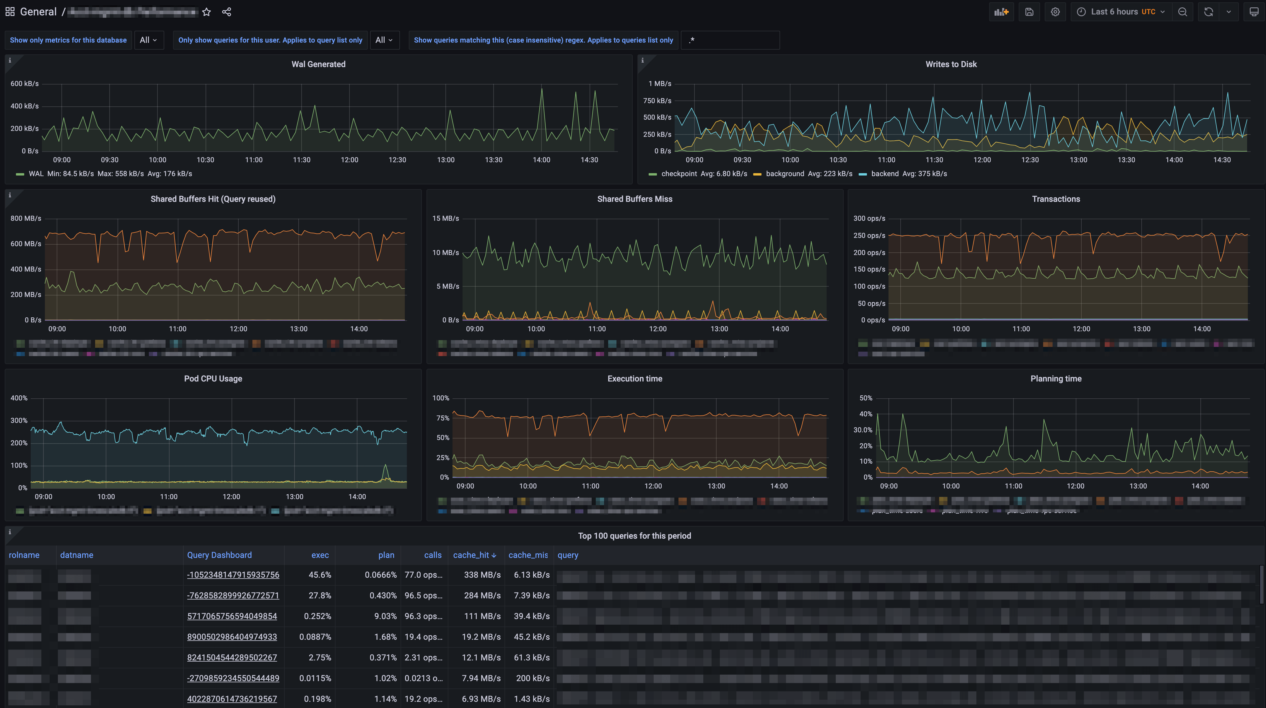
Top 100 most expensive queries
Getting an overview of the cluster instance is really helpful to understand the state of the whole system over time. Another useful set of data to analyze quickly is a list of the queries using the most resources of the cluster, query by query. There are many ways you could query the snapshot information for these details, and your definition of "resource-intensive" might be different than what we show, but this example gives the high-level cumulative statistics for each query over the specified time, ordered by the highest total sum of execution and planning time.
/*
* individual data for each query for a specified time range,
* which is particularly useful for zeroing in on a specific
* query in a tool like Grafana
*/
WITH snapshots AS (
    SELECT
        max,
        -- We need at least 2 snapshots to calculate a delta. If the dashboard is currently showing
        -- a period < 5 minutes, we only have 1 snapshot, and therefore no delta. In that CASE
        -- we take the snapshot just before this window to still come up with useful deltas
        CASE
            WHEN max = min
THEN (SELECT max(created) FROM statements_history.snapshots WHERE created < min)
            ELSE min
        END AS min
    FROM (
        SELECT
            max(created),
            min(created)
        FROM
            statements_history.snapshots WHERE created > now() - '1 hour'::interval
            -- Grafana-based filter
            --statements_history.snapshots WHERE $__timeFilter(created)
        GROUP by
            stats_reset
        ORDER by
            max(created) DESC
        LIMIT 1
    ) AS max(max, min)
), deltas AS (
    SELECT
        rolname,
        datname,
        queryid,
        extract('epoch' from max(created) - min(created)) AS delta_seconds,
        max(total_exec_time) - min(total_exec_time) AS delta_exec_time,
        max(total_plan_time) - min(total_plan_time) AS delta_plan_time,
        max(calls) - min(calls) AS delta_calls,
        max(shared_blks_hit) - min(shared_blks_hit) AS delta_shared_blks_hit,
        max(shared_blks_read) - min(shared_blks_read) AS delta_shared_blks_read
    FROM
        statements_history.statements
    WHERE
 -- granted, this looks odd, however it helps the DecompressChunk Node tremendously,
        -- as without these distinct filters, it would aggregate first and then filter.
        -- Now it filters while scanning, which has a huge knock-on effect on the upper
        -- Nodes
        (created >= (SELECT min FROM snapshots) AND created <= (SELECT max FROM snapshots))
    GROUP BY
        rolname,
        datname,
        queryid
)
SELECT
    rolname,
    datname,
    queryid::text,
    delta_exec_time/delta_seconds/1000 AS exec,
    delta_plan_time/delta_seconds/1000 AS plan,
    delta_calls/delta_seconds AS calls,
    delta_shared_blks_hit/delta_seconds*8192 AS cache_hit,
    delta_shared_blks_read/delta_seconds*8192 AS cache_miss,
    query
FROM
    deltas
JOIN
    statements_history.queries USING (rolname,datname,queryid)
WHERE
    delta_calls > 1
    AND delta_exec_time > 1
    AND query ~* $$.*$$
ORDER BY
    delta_exec_time+delta_plan_time DESC
LIMIT 100;


rolname  |datname|queryid             |exec              |plan|calls               |cache_hit         |cache_miss|query
---------+-------+--------------------+------------------+----+--------------------+------------------+----------+-----------
tsdbadmin|tsdb   |731301775676660043  |0.0000934033977289| 0.0|0.016660922907623773| 228797.2725854585|       0.0|WITH statem...
tsdbadmin|tsdb   |-686339673194700075 |0.0000570625206738| 0.0|  0.0005647770477161|116635.62329618855|       0.0|WITH snapsh...
tsdbadmin|tsdb   |-5804362417446225640|0.0000008223159463| 0.0|  0.0005647770477161| 786.5311077312939|       0.0|-- NOTE Thi...
However you decide to order this data, you now have a quick result set with the text of the query and the queryid. With just a bit more effort, we can dig even deeper into the performance of a specific query over time.
For example, in the output from the previous query, we can see that queryid=731301775676660043 has the longest overall execution and planning time of all queries for this period. We can use that queryid to dig a little deeper into the snapshot-by-snapshot performance of this specific query.
/*
 * When you want to dig into an individual query, this takes
 * a similar approach to the "snapshot" query above, but for
 * an individual query ID.
 */
WITH deltas AS (
    SELECT
        created,
        st.calls - lag(st.calls) OVER (query_w) AS delta_calls,
        st.plans - lag(st.plans) OVER (query_w) AS delta_plans,
        st.rows - lag(st.rows) OVER (query_w) AS delta_rows,
        st.shared_blks_hit - lag(st.shared_blks_hit) OVER (query_w) AS delta_shared_blks_hit,
        st.shared_blks_read - lag(st.shared_blks_read) OVER (query_w) AS delta_shared_blks_read,
        st.temp_blks_written - lag(st.temp_blks_written) OVER (query_w) AS delta_temp_blks_written,
        st.total_exec_time - lag(st.total_exec_time) OVER (query_w) AS delta_total_exec_time,
        st.total_plan_time - lag(st.total_plan_time) OVER (query_w) AS delta_total_plan_time,
st.wal_bytes - lag(st.wal_bytes) OVER (query_w) AS delta_wal_bytes,
        extract('epoch' from st.created - lag(st.created) OVER (query_w)) AS delta_seconds
    FROM
        statements_history.statements AS st
    join
        statements_history.snapshots USING (created)
    WHERE
        -- Adjust filters to match your queryid and time range
        created > now() - interval '25 minutes'
        AND created < now() + interval '25 minutes'
        AND queryid=731301775676660043
    WINDOW
        query_w AS (PARTITION BY datname, rolname, queryid, stats_reset ORDER BY created)
)
SELECT
    created AS "time",
    delta_calls/delta_seconds AS calls,
    delta_plans/delta_seconds AS plans,
    delta_total_exec_time/delta_seconds/1000 AS exec_time,
    delta_total_plan_time/delta_seconds/1000 AS plan_time,
    delta_rows/nullif(delta_calls, 0) AS rows_per_query,
    delta_shared_blks_hit/delta_seconds*8192 AS cache_hit,
    delta_shared_blks_read/delta_seconds*8192 AS cache_miss,
    delta_temp_blks_written/delta_seconds*8192 AS temp_bytes,
    delta_wal_bytes/delta_seconds AS wal_bytes,
    delta_total_exec_time/nullif(delta_calls, 0) exec_time_per_query,
    delta_total_plan_time/nullif(delta_plans, 0) AS plan_time_per_plan,
    delta_shared_blks_hit/nullif(delta_calls, 0)*8192 AS cache_hit_per_query,
    delta_shared_blks_read/nullif(delta_calls, 0)*8192 AS cache_miss_per_query,
    delta_temp_blks_written/nullif(delta_calls, 0)*8192 AS temp_bytes_written_per_query,
    delta_wal_bytes/nullif(delta_calls, 0) AS wal_bytes_per_query
FROM
    deltas
WHERE
    delta_calls > 0
ORDER BY
    created ASC;


time                         |calls               |plans|exec_time         |plan_time|ro...
-----------------------------+--------------------+-----+------------------+---------+--
2022-04-14 14:33:39.831 -0400|0.016662115132216382|  0.0|0.0000735602224659|      0.0|
2022-04-14 14:34:39.847 -0400|0.016662248949061972|  0.0|0.0000731468396678|      0.0|
2022-04-14 14:35:39.863 -0400|  0.0166622286820572|  0.0|0.0000712116494436|      0.0|
2022-04-14 14:36:39.880 -0400|0.016662015187426844|  0.0|0.0000702374920336|      0.0|
Compression, Continuous Aggregates, and Data Retention
This self-serve query monitoring setup doesn't require TimescaleDB. You could schedule the snapshot job with other extensions or tools, and regular PostgreSQL tables could likely store the data you retain for some time without much of an issue. Still, all of this is classic time-series data, tracking the state of your PostgreSQL cluster(s) over time.
Keeping as much historical data as possible provides significant value to this database monitoring solution's effectiveness. TimescaleDB offers several features that are not available with vanilla PostgreSQL to help you manage growing time-series data and improve the efficiency of your queries and process.
Compression on this data is highly effective and efficient for two reasons:
- Most of the data is stored as integers which compresses very well (96 % plus) using our type-specific algorithms.
- The data can be compressed more frequently because we're never updating or deleting compressed data. This means that it's possible to store months or years of data with very little disk utilization, and queries on specific columns of data will often be significantly faster from compressed data.
Continuous aggregates allow you to maintain higher-level rollups over time for aggregate queries that you run often. Suppose you have dashboards that show 10-minute averages for all of this data. In that case, you could write a continuous aggregate to pre-aggregate that data for you over time without modifying the snapshot process. This allows you to create new aggregations after the raw data has been stored and new query opportunities come to light.
And finally, data retention allows you to drop older raw data automatically once it has reached a defined age. If continuous aggregates are defined on the raw data, it will continue to show the aggregated data which provides a complete solution for maintaining the level of data fidelity you need as data ages.
These additional features provide a complete solution for storing lots of monitoring data about your cluster(s) over the long haul. See the links provided for each feature for more information.
Better Self-Serve Query Monitoring With pg_stat_statements
Everything we've discussed and shown in this post is just the beginning. With a few hypertables and queries, the cumulative data from pg_stat_statementscan quickly come to life. Once the process is in place and you get more comfortable querying it, visualizing it will be very helpful.

pg_stat_statements is automatically enabled in all Timescale services. If you’re not a user yet, you can try out Timescale for free (no credit card required) to get access to a modern cloud-native database platform with TimescaleDB's top performance.
To complement pg_stat_statements for better query monitoring, check out Insights, also available for trial services.


