Creating a Fast Time-Series Graph With Postgres Materialized Views

Imagine you have a massive amount of time-series data you want to explore and visualize. Seeing the latest trends, the historical patterns, and the outliers in your data can help you gain insights and make decisions. But how do you visualize and analyze time-series data effectively? How do you create graphs, plots, and other visualizations for real-time analytics showing the current state of your data and the historical changes over different time intervals? And how do you do it efficiently without sacrificing performance or accuracy?
In this article, we will see how to use PostgreSQL materialized views and Timescale’s improved version of these—continuous aggregates—to create a time-series graph that answers these questions.
Creating a Time-Series Graph in PostgreSQL
Method 1: Creating plots and graphs directly from raw data
Pretend you are a senior engineer at a company that creates devices to monitor the electrical power grid. These devices export a large amount of data—one PostgreSQL row is created per device every second. For this example, let's say the local power company uses one hundred devices (60,480,000 rows created per week). You want to be able to give your customers data visualizations of the load on a given line per hour, day, and week.
Our table looks like this:
CREATE TABLE demand (
    id          serial primary key,
    amps        DOUBLE PRECISION  NOT NULL,
    location    TEXT,
    time        TIMESTAMPTZ       NOT NULL
);
We can import a single device's data by running the following INSERT command (or, you know, generate dummy data!). It will take some time to insert 10,540,800 rows; shorten the gap between timestamps to produce less data:
INSERT INTO demand (amps, location, time) VALUES  (random()*40, 'Spokane, WA',
generate_series('2023-09-01T00:00:00+03:00'::timestamptz, '2023-12-31T23:59:59+03:00'::timestamptz, '1 second'));
Now, we can generate a time-series plot to calculate average amps per minute with the following SQL. Change '1 minute' to '1 day' or '1 week' to create time-series plots for different intervals.
SELECT
 date_bin(interval '1 minute', time, timestamptz '2023-08-01' ) AS time_interval,
 AVG(amps)
FROM demand
GROUP BY 1
ORDER BY 1;
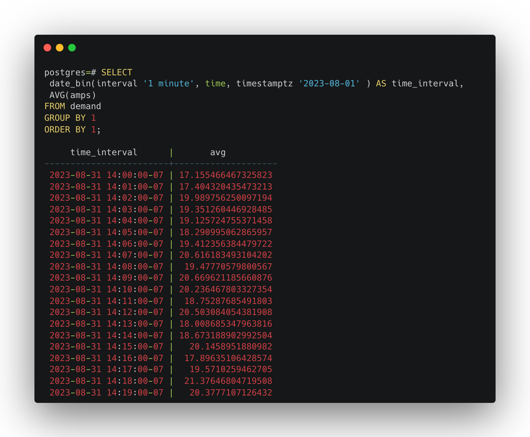
This query can take some time, depending on how much data is in the demand table. For the 10,540,800 rows we created, the query takes 15 seconds to execute on an 8-Core Intel Core i9 with 32 GB RAM Apple MacBook Pro. That is 15 seconds to return plot data for a single device over three months! Imagine if we had hundreds or thousands of devices spanning over a year.
Let's look at a few ways to improve the speed of our time-series plot using materialized views and continuous aggregates.
Method 2: Using materialized views to make graphs more performant
In PostgreSQL, a view can be thought of as a stored query on top of a table. When we query a view, the underlying query the view was created with gets called. This gives us the ability to abstract away and simplify our queries, but a view won't do much to improve the speed of a query.
Somewhere between a table and a view sits the materialized view. A materialized view works similarly to a view in that you can make queries reusable. The difference is a materialized view will store the resulting data on disk—caching the data. When you use a materialized view, you don’t have to run the query again. You get the results from the disk. This makes your queries much faster!
To improve the speed of our time-series graph data, let's create a materialized view over the demand table.
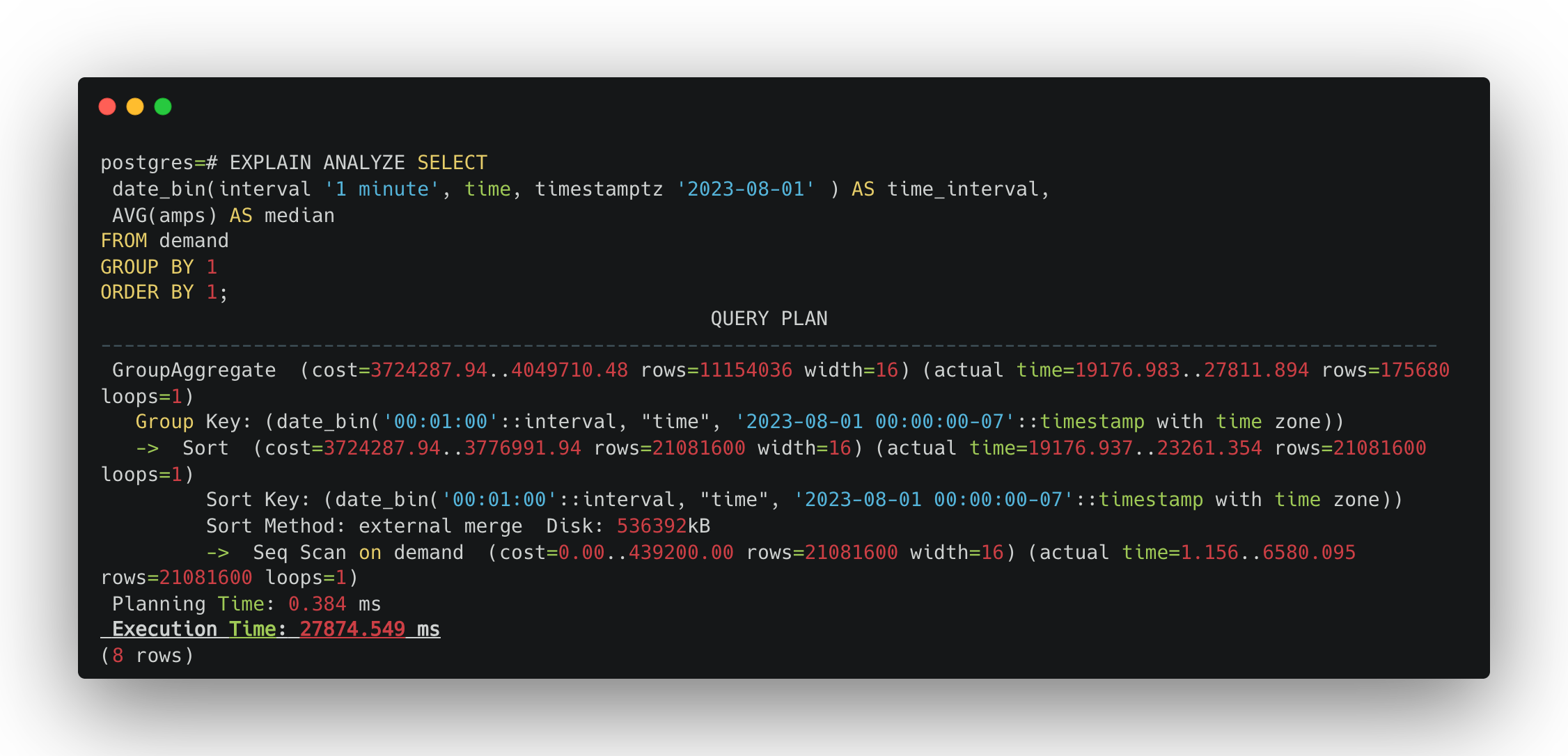
CREATE MATERIALIZED VIEW demand_amps_by_minute AS
SELECT
  date_bin(
    interval '1 minute', time, timestamptz '2023-08-01'
  ) AS time_interval,
  AVG(amps) AS median
FROM
  demand
GROUP BY
  1
ORDER BY
  1;
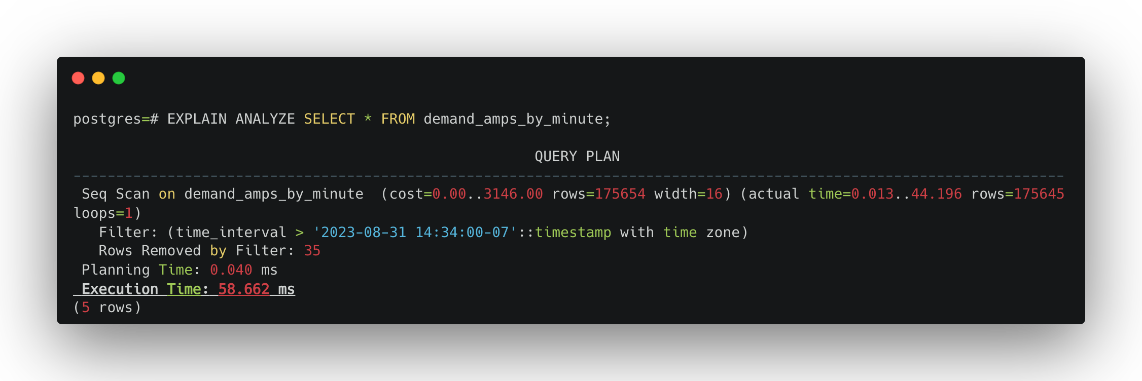
Since creating the materialized view needs to run the same average amps per minute SQL, it can take some time to create. Once it's complete, run SELECT * FROM demand_amps_by_minute;. On my same MacBook Pro, the query now takes 58ms—much better!
This shows off the speed improvement materialized views can give us, but they come with a downside we haven't covered yet. When new data is added, updated, or deleted from the underlying table, we have to manually refresh the materialized view with a REFRESH MATERIALIZED VIEW [materialized view name]; statement. This will completely replace the data in the materialized view with all the new data from the table using the query from the definition.
Having to refresh your materialized views comes with a few glaring problems:
- If you have a steady stream of data being written to your table, which is very common in time-series data, then once you refresh your materialized view, it'll be out of date.
- Refreshing a materialized view comes with a performance hit, as it needs to rerun the materialized view's definition on all the data in the table to refresh itself.
- You'll need to remember to manually run a refresh on your materialized views or maintain a cron job.
However, Timescale has engineered a little magic under the hood to remove all these pain points of using materialized views through continuous aggregates.
Method 3: Creating graphs that are more resource-efficient and easier to maintain via continuous aggregates
Timescale’s continuous aggregates have the same look and feel as materialized views, but they add some essential functionality to help you keep your graphs, plots, dashboards, or other visualizations of real-time analytics performant over time without manual maintenance.
First, continuous aggregates stay automatically updated via a refresh policy defined by you—i.e., you can configure your continuous aggregate view so it gets updated automatically every 30 minutes, including your latest data. This is much more convenient than refreshing your views manually!
But the key is what happens under the hood once this refresh policy kicks in. In plain PostgreSQL materialized views, when you refresh the view, the query will be recomputed over the entire dataset. In other words, in plain PostgreSQL, materialized views’ refreshes are not incremental. This makes the refresh process computationally expensive unnecessarily, especially once your dataset grows and a large volume of data needs to be materialized.
Continuous aggregates fix this inefficiency: when you refresh a continuous aggregate, Timescale doesn’t drop all the old data and recompute the aggregate against it. Instead, the engine just runs the query against the most recent refresh period (e.g., 30 minutes) and the data that has changed since the last refresh. This way, continuous aggregates keep your visualizations performant over time, independently of how much your dataset is growing.
Switching over to Timescale, we'll recreate our demand table using the same CREATE TABLE statement as before but leaving off the id column (we'll use time instead).
CREATE TABLE demand (
    amps        DOUBLE PRECISION  NOT NULL,
    location    TEXT,
    time        TIMESTAMPTZ       NOT NULL
);
Next, we'll update demand to be a hypertable:
SELECT create_hypertable('demand', 'time');
Finally, populate the demand table with data:
INSERT INTO demand (amps, location, time) VALUES  (random()*40, 'Spokane, WA',
generate_series('2023-09-01T00:00:00+03:00'::timestamptz, '2023-12-31T23:59:59+03:00'::timestamptz, '1 second'));
At last we can create our continuous aggregate that will work similarly to the previous materialized view.
CREATE MATERIALIZED VIEW demand_amps_by_minute
WITH (timescaledb.continuous) AS
SELECT
   time_bucket(INTERVAL '1 minute', time) AS bucket,
   AVG(amps)
FROM demand
GROUP BY bucket;
We need to update its refresh policy to have our continuous aggregate continuously refresh. For this example, we'll have it refresh every minute. But for your own workloads, you'll need to optimize these settings to fit your needs.
SELECT add_continuous_aggregate_policy(
	'demand_amps_by_minute',
	start_offset => NULL,
	end_offset => INTERVAL '1 h',
	schedule_interval => INTERVAL '1 m');
If we run a SELECT query on demand_amps_by_minute, I now get 120 ms to query the continuous aggregate. A little bit slower than a raw materialized view, but we're still much faster than querying the table!
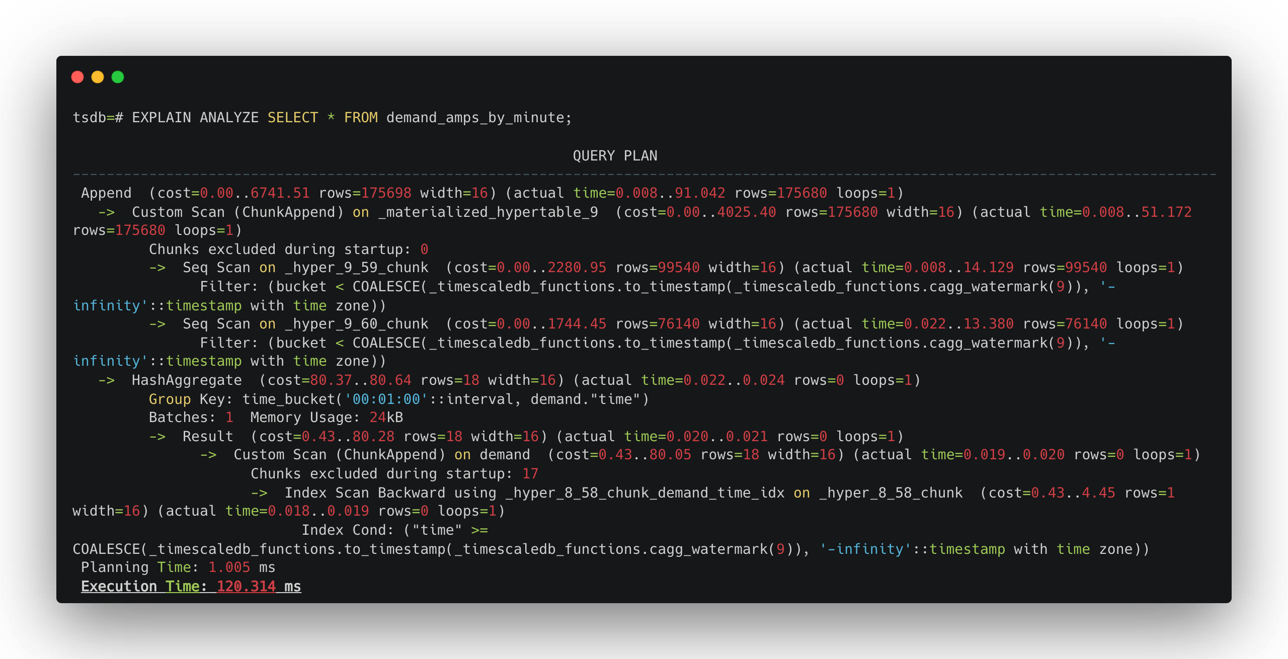
Continuous aggregates track which chunks have been materialized and what data hasn't been yet by using a watermark (e.g., a pointer). When you query a continuous aggregate, you get materialized data before the watermark and non-materialized data after the watermark. This watermark will move as the aggregate policy continues to work through materializing non-materialized data.
All this adds some time to the overall query speed, but we benefit from not having to manually refresh the materialized view!
Let's try it out. Insert a new row into the underlying demand table.
INSERT INTO demand (amps, location, time) VALUES (100.2, 'Pullman, WA', now())
Then, if we re-query our continuous aggregate, we'll see the newly added row returned to us.
Start Speeding Up Your Queries Today
Throughout this article, we discovered how to use a table to create a time-series graph for large amounts of data. We improved the query performance by taking advantage of PostgreSQL's materialized views.
However, materialized views can be time-consuming to maintain. Last, we removed the need to manually refresh the materialized view by taking advantage of Timescale's continuous aggregates. Now, it’s your turn to create your own time-series plots or real-time analytics using these methods!
You can create a free Timescale account and start speeding up your queries today.