What Is Distributed Tracing and How Jaeger Tracing Is Solving Its Challenges
With the increased adoption of distributed systems, where many system components are located on different machines, it has become both more important and more difficult to monitor these systems effectively. As more things can go wrong, quickly identifying and solving them can mean the difference between success and failure.
That fine line has been driving the rapid adoption growth for popular technologies such as Jaeger and OpenTelemetry. These tools/libraries provide insight into how your application operates and performs through distributed tracing, allowing developers to see how the application requests are handled across their distributed systems. But more on that later.
A popular tool for distributed tracing is Jaeger, which introduced a new experimental feature called Service Performance Monitoring earlier this year. As the name suggests, this feature adds performance monitoring to your traditional distributed tracing tool.
This blog post will discuss what problem this feature solves and why it is a welcome addition to Jaeger. On top of that, we will take a deep look at how the OpenTelemetry Collector interacts with Jaeger to aggregate traces into Prometheus metrics and neatly graph them inside Jaeger’s UI.
Let’s get started.
What Is Distributed Tracing?
First, let’s go back quickly to distributed tracing. Distributed tracing is the process of following and measuring requests through your system as they flow from microservice to microservice or frontend mobile application to your backend or from a microservice to a database.
Spans are the data collected from distributed tracing inter-service requests and contain a wide range of information about the request. The group of spans that originates from the same initial request is called a trace.
How Do Spans and Traces Work?
Traces are propagated between services through metadata attached to the request, which we call context. When a request first enters a distributed system, your instrumentation (most likely OpenTelemetry) creates a root span. All subsequent requests between microservices will create a child span with a context that contains the following information:
- Its own ID
- The ID of the root span
- The ID of its parent span
- Some timestamps and other logs
If you start at the root span and follow the child ID of every span until you reach a leaf span (a span with no children), much like a binary tree, you can accurately reconstruct the services your request/trace has reached without having to collect the traces in order.
Doing it this way suits a distributed system much better as the instrumentation doesn’t need to wait for confirmation that the parent span has been written to a persistent store, nor does it needs to know about spans being instrumented simultaneously.
The Challenges of Distributed Tracing
Usually, you combine tracing with more traditional logging and metrics instrumentation. Still, due to the breadth and depth of traces, you can extrapolate a wide variety of helpful information from those traces. Each span (and therefore trace) starts with a timestamp from which you can calculate the total amount of time each request took.
A well-instrumented tracing system ensures that if any event or error occurs, it gets stored in the context of said span. When following the spans from the root spans to the leaf spans, you can summate the number of errors (or lack thereof) within your request’s lifetime. When looking at all collected traces, you can calculate the total number of traces generated in a set timeframe and the percentage of erroneous requests.
While this can provide an accurate view of what is going on inside your distributed system, it is computationally expensive to iterate through thousands (if not hundreds of thousands) of traces—each of which can contain hundreds of spans—to calculate a single metric.
A dashboard with automatic refresh functionality will make it, but it will unnecessarily slow down your metrics store's insert and collection performance. Why? You will have to reread all traces within a certain time frame from your database and recalculate all metrics with the newly collected traces (a majority of which had already been calculated in the previous refresh).
Another problem is that since trace data is produced in such huge volumes, it is commonplace to only instrument a set percentage of requests. This is called “sampling” and provides a way to balance the observability of a system and the computational expense of tracing. If our sampling rate is set at 15 percent, we only trace 15 out of 100 requests, for example.
This is a problem for the accuracy of the metrics deducted from these traces, as it will skew our final results. And it is even more so when doing tail-based sampling, where we wait until the trace has been completed before sampling to decide to keep traces with high latency or where an error occurs. While unlikely, those 15 traces may contain an error.
In that case, our dashboard would report a 100 percent error rate, even though the 85 other requests could be perfectly fine. Seeing inaccurate metrics during a crisis can lead to a higher MTTR and more error-prone debugging, which is undesirable, to say the least!
A great way to circumvent skewing our service performance metrics is by aggregating the metrics of a collection of traces after they have been completed and before sampling is applied. Doing it this way ensures an accurate result, even if we don’t keep all the traces.
Another added benefit is that the processing happens as the traces are generated instead of when they are queried. This prevents your storage backend from overloading when you query the service performance metrics. Where the storage backend would have to read each span of each trace and aggregate it in real time, it can now just return the pre-aggregated metrics.
What Is Jaeger's Service Performance Monitoring?
Now, let’s see how Jaeger, a renowned tool for distributed tracing, is solving these challenges to provide accurate service performance metrics.
Traditionally, Jaeger has only allowed storing, querying, and visualizing individual traces, which is great for troubleshooting a specific problem but not useful for getting a general sense of how well your services perform. That was until they introduced, earlier this year, a new experimental feature called Service Performance Monitoring (SPM).
To use the SPM feature within the Jaeger UI, you are required to use the OpenTelemetry Collector to collect traces and a Prometheus-compatible backend. Traces enter the OpenTelemetry Collector at one of two trace receivers: OpenTelemetry or Jaeger, depending on the configuration.
From there, they are sent to the configured processors. In our case, these are the Spanmetrics Processor and Batch Processor. The appropriate trace exporter exports the metrics (as usual) to a Jaeger- or OpenTelemetry-compatible trace storage backend.
The Spanmetrics Processor calculates the metrics, and then you use the Prometheus or the PrometheusRemoteWrite exporter to get the metrics into a Prometheus-compatible backend.
Below is an architecture diagram of the solution and how spans and metrics flow through the system.

How the Spanmetrics Processor Works
The Spanmetrics Processor receives spans and computes aggregated metrics from them.
It creates four Prometheus metrics:
calls_total: The calls_total metrics is a counter which counts the total number of spans per unique set of dimensions. You can identify the number of errors by thestatus_codelabel. You can use it to calculate the percentage of erroneous calls by dividing the metrics that contain astatus_codelabel equal toSTATUS_CODE_ERRORby the total number of metrics and multiplying it by 100.
This is an example of the PromQL metrics exposed for the calls_total metric:
calls_total{operation="/", service_name="digit", span_kind="SPAN_KIND_SERVER", status_code="STATUS_CODE_UNSET"}
30255
calls_total{operation="/", service_name="special", span_kind="SPAN_KIND_SERVER", status_code="STATUS_CODE_ERROR"}
84
calls_total{operation="/", service_name="upper", span_kind="SPAN_KIND_SERVER", status_code="STATUS_CODE_UNSET"}
15110
calls_total{operation="GET /", service_name="lower", span_kind="SPAN_KIND_SERVER", status_code="STATUS_CODE_UNSET"}
15085
latency: This metric is made up of multiple underlying Prometheus metrics that combined represent a histogram. Because of the labels attached to these metrics, you can create histograms for latency on a per operation or service level.latency_count: thelatency_countcontains the total amount of data points in the buckets.
latency_count{operation="/", service_name="digit", span_kind="SPAN_KIND_SERVER", status_code="STATUS_CODE_UNSET"}
32278
latency_count{operation="/", service_name="special", span_kind="SPAN_KIND_SERVER", status_code="STATUS_CODE_ERROR"}
88
latency_count{operation="/", service_name="upper", span_kind="SPAN_KIND_SERVER", status_code="STATUS_CODE_ERROR"}
87
latency_count{operation="/", service_name="upper", span_kind="SPAN_KIND_SERVER", status_code="STATUS_CODE_UNSET"}
16109
latency_sum: thelatency_sumcontains the sum of all the data point values in the buckets.
latency_sum{operation="/", service_name="digit", span_kind="SPAN_KIND_SERVER", status_code="STATUS_CODE_UNSET"}
8789319.72
latency_sum{operation="/", service_name="special", span_kind="SPAN_KIND_SERVER", status_code="STATUS_CODE_ERROR"}
991.98
latency_sum{operation="/", service_name="upper", span_kind="SPAN_KIND_SERVER", status_code="STATUS_CODE_ERROR"}
1087.28
latency_sum{operation="/", service_name="upper", span_kind="SPAN_KIND_SERVER", status_code="STATUS_CODE_UNSET"}
1060574.74
latency_bucket: The latency_bucket contains the number of data points where the latency is less than or equal to a predefined time. You can configure the granularity (or amount of buckets) by changing the latency_histogram_buckets array in your OpenTelemetry Collector configuration.
latency_bucket{le="+Inf", operation="/", service_name="digit", span_kind="SPAN_KIND_SERVER", status_code="STATUS_CODE_UNSET"}
32624
latency_bucket{le="+Inf", operation="/", service_name="special", span_kind="SPAN_KIND_SERVER", status_code="STATUS_CODE_ERROR"}
90
latency_bucket{le="+Inf", operation="/", service_name="special", span_kind="SPAN_KIND_SERVER", status_code="STATUS_CODE_UNSET"}
16150
latency_bucket{le="+Inf", operation="/", service_name="upper", span_kind="SPAN_KIND_SERVER", status_code="STATUS_CODE_ERROR"}
88
Learn more about the different types of Prometheus metrics in this blog post.
How to Query the Prometheus Metrics
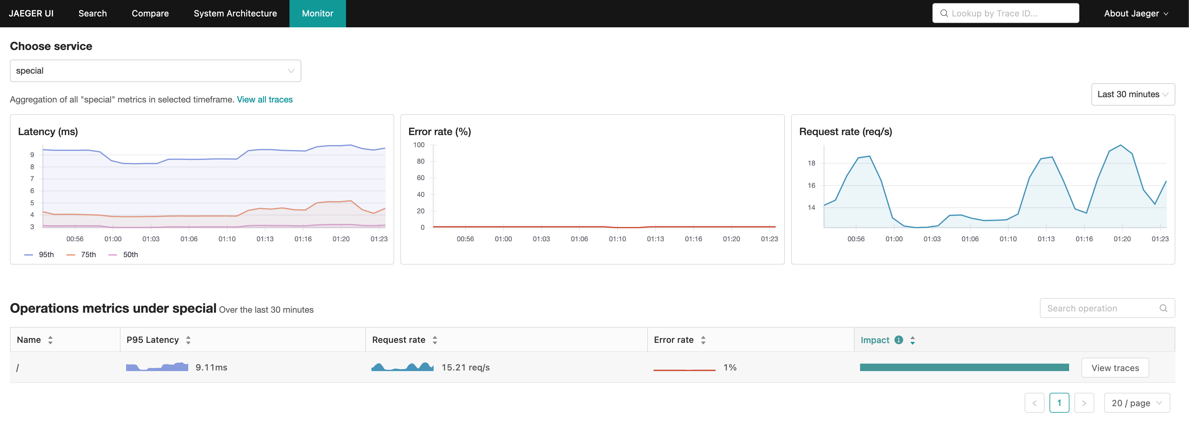
You can aggregate the Prometheus metrics mentioned above into RED metrics: RED stands for Rate, Error, and Duration. You can use these three metrics to identify slow and erroneous services within your distributed system.
The Jaeger UI queries these metrics from Prometheus and visualizes them in three distinct service-level graphs. Latency (duration), Error rate (error), and Request rate (rate). On top of that, the Jaeger UI also presents you with these metrics per operation for the selected service.

Because of its relative simplicity and lack of fine-grained controls, Jaeger’s SPM doesn’t eliminate the need for a more conventional metrics collection infrastructure and custom Grafana dashboards. But it should definitely be the first destination for anyone wanting to see what is going on in their distributed system at a glance on a per-service basis.
Building on SPM: Creating Custom Instrumentation for Jaeger Distributed Tracing Using Grafana
Since these RED metrics are stored in a Prometheus-compatible storage backend, you can also query them outside the Jaeger UI. This is great if you combine these metrics with other custom instrumentation inside a Grafana dashboard.
The following PromQL query gives us a simple overview of the request rate of all our services in a single Grafana panel:
sum(rate(calls_total[1m])) by (service_name)

Combining the following PromQL queries gives us a comprehensive view of the latency on a per percentile basis. By adding a variable in your Grafana dashboard, you can make it easier to switch between services.
histogram_quantile(0.50, sum(rate(latency_bucket{service_name =~ "generator"}[1m])) by (service_name, le))
histogram_quantile(0.90, sum(rate(latency_bucket{service_name =~ "generator"}[1m])) by (service_name, le))
histogram_quantile(0.95, sum(rate(latency_bucket{service_name =~ "generator"}[1m])) by (service_name, le))

The Verdict: How Jaeger's SPM Changes Distributed Tracing
In conclusion, Jaeger’s SPM feature is a welcome addition to the Jaeger UI. It provides easy access to RED metrics aggregated from traces you are already collecting.
It is a great place to start troubleshooting your distributed system as it gives you a high-level overview of your service-level operations and the option to jump directly into Jaeger's Tracing tab on the operation of your choice for more detailed analysis. If you are already using the OpenTelemetry Collector to collect and process metrics and traces, enabling this feature is a no-brainer that takes no less than 10 minutes to configure.
A way to further ease this transition is to store your metrics and traces in the same unified location. Operating and managing just a single storage backend reduces architectural complexity and operational overhead. Additionally, you benefit from correlating metrics and traces much more efficiently as they are stored in one place.