SQL vs. Flux: Choosing the right query language for time-series data
An examination of the strengths and weaknesses of SQL, and why query planners exist, by way of comparing TimescaleDB and InfluxDB.
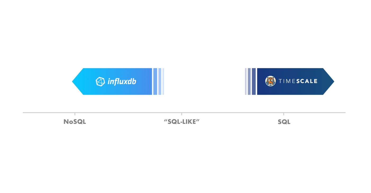
Generally in the world of database query languages, there have been two extremes: full SQL support on one end, and completely custom languages (sometimes known as “NoSQL”) on the other.

With time-series databases, the differences between these languages can be seen by comparing TimescaleDB and InfluxDB.
From the beginning, TimescaleDB has firmly existed at the SQL end of the spectrum, fully embracing the language from day 1, and later further extending it to simplify time-series analysis. This has enabled TimescaleDB to require a zero learning curve for new users, and allowed it to inherit the entire SQL ecosystem of 3rd party tools, connectors, and visualization options, which is larger than that of any other time-series database.
In contrast, InfluxDB began with a “SQL-like” query language (called InfluxQL), placing it in the middle of the spectrum, and has recently made a marked move towards the “custom” end with its new Flux query language. This has allowed InfluxDB to create a new query language that its creators would argue overcomes some SQL shortcomings that they experienced. (Read the Flux announcement and the Hacker News reaction.)
So how do these two query languages compare?
To analyze the differences between SQL and Flux, let’s first dig into why the InfluxDB team created Flux, as opposed to embracing SQL.
According to this post, InfluxDB created Flux primarily for two reasons:
- Query support: They concluded SQL could not easily handle the types of queries they wanted to run on time-series data.
- Relational algebra vs. flow-based functional processing: They believed that a time-series query language needed a flow-based functional model, as opposed to the relational algebra model in SQL.
(There’s also a third reason stated in the post: that SQL was invented in the 1970s. This point is odd, especially considering that other foundational technologies were also born in that same era: the relational database, the microprocessor, and the Internet. These technologies, like SQL, have evolved significantly since their initial invention, while other technologies have not. Also, common modern languages such as English were “invented” hundreds of years ago, and have also evolved over time, while other languages have fallen out of use. So we believe the decade in which something was invented is irrelevant to this discussion. With that in mind, we’ll return to the main discussion.)
Let’s unpack both of these reasons.
Query support
Here’s the canonical example InfluxDB uses in their post, which computes an exponential moving average (EMA), to support their claim:
Flux:
from(db:"telegraf")
|> range(start:-1h)
|> filter(fn: (r) => r._measurement == "foo")
|> exponentialMovingAverage(size:-10s)
The post authors then struggle to write this query in SQL, and instead produce a fairly complex query that computes a simple moving average:
SQL 1:
select id,
       temp,
       avg(temp) over (partition by group_nr order by time_read) as rolling_avg
from (
  select id,
         temp,
         time_read,
         interval_group,
         id - row_number() over (partition by interval_group order by time_read) as group_nr
  from (
     select id,
            time_read,
            'epoch'::timestamp + '900 seconds'::interval * (extract(epoch from time_read)::int4 / 900) as interval_group,
            temp
     from readings
  ) t1
) t2
order by time_read;
Yes, this SQL example is quite verbose, and only computes part of the desired output (i.e., it only computes a moving average, not an exponential moving average). As a result, their argument is that common time-series related queries (such as computing an EMA) are quite complex in SQL.
We find this argument incorrect for a key reason. The only way that Flux could support this function is if its creators wrote their own exponentialMovingAverage() function.
One can similarly write the same function in modern SQL, by creating a custom aggregate. Creating a custom aggregate is supported in most modern SQL implementations, including PostgreSQL. The syntax in PostgreSQL is the following (via StackOverflow):
SQL: Creating the custom aggregate
CREATE OR REPLACE FUNCTION exponential_moving_average_sfunc
(state numeric, next_value numeric, alpha numeric)
RETURNS numeric LANGUAGE SQL AS
$$
SELECT
         CASE
                WHEN state IS NULL THEN next_value
                ELSE alpha * next_value + (1-alpha) * state
         END
$$;
CREATE AGGREGATE exponential_moving_average(numeric, numeric)
(sfunc = exponential_moving_average_sfunc, stype = numeric);
(This is a simple SQL aggregate window function that computes the exponential moving average. It is an aggregate function because it takes multiple input rows, and is a window function because it computes a value for each input row. By comparison, computing a regular SUM would be an aggregate but not a window function, while comparing the delta between two rows would be a window function but not an aggregate. Yes, SQL is powerful.)
Then querying for the exponential moving average of the entire dataset can be rather simple:
SQL 2:
SELECT time,
       exponential_moving_average(value, 0.5) OVER (ORDER BY time)
FROM telegraph
WHERE measurement = 'foo' and time > now() - '1 hour';
This function also allows you to calculate the EMA not just across time, but also by any other column (e.g., “symbol”). In the following example, we calculate the EMA for each different stock symbol over time:
SQL 3:
SELECT date,
       symbol,
       exponential_moving_average(volume, 0.5) OVER (
         PARTITION BY symbol ORDER BY date ASC)
FROM telegraph
WHERE measurement = 'foo' and time > now() - '1 hour'
ORDER BY date, symbol;
(You can see more at this SQL Fiddle.)
Yes, writing a new function requires some work, but less work than learning a whole new language, not to mention forcing everyone else (who could just use the same function) to learn that language.
As developers of a database, we would also argue that writing a new SQL function requires far less work than writing a new query language from scratch. Especially when you consider that even after writing the language, one would still need to write that same specific function (which is what the Flux creators have done).
Given the large corpus of prior efforts in SQL to perform tasks like calculating an EMA (such as StackOverflow), and given the extensibility of SQL, we would also argue that spending more time in SQL would be a better return on investment than learning or even developing a new query language from scratch, let alone forcing all future database users to also learn that language.
What about verbosity?
One could argue that the Flux syntax is slightly less verbose than the SQL syntax. But forcing users to learn a new query language so they can save a few keystrokes when writing their queries feels like the wrong trade-off. Programming language complexity is not really about the number of keystrokes one types, but the mental burden to do so: for example, a 1 line program in one language might in fact be more difficult and time-consuming to write (and maintain) than a 5 line program in another language.
What about the SQL standard?
One could also argue that creating new functions (or aggregates) breaks the SQL standard. Having a standard is valuable for two reasons: code portability, and skills re-use. Here we find that extending SQL is still a superior path than using a new query language. While creating new functions in SQL reduces code portability, it does so far less than adopting a non-standard language. And because the new function syntax is quite similar (if not equivalent) to the standard, it allows database users to leverage their existing knowledge from other systems, which would not be possible with a non-standard language. And SQL’s extensibility allows you to mold the language around your problem domain.
Relational algebra vs. flow-based functional processing
The other reason InfluxDB cites for developing Flux is that they wanted a language that processed data in a flow-based functional model, versus SQL which is based on relational algebra and sets.
For example, the Flux creators wanted to easily chain query processing steps in an incremental way. Their argument is that chaining operations and building incremental queries is not easy in SQL. In Flux, this chaining is established by the pipe-forward (“|>“) operator. Flux also allows for arbitrary code to be run in each step of the pipeline (e.g. the filter operator in their example above).
We find that this argument has some merit, but not without trade-offs.
First, we agree that writing incremental queries in SQL is not as easy as chaining the output from one function into another (although sub-SELECTs and Common Table Expressions make this easier). Updating a query typically requires some re-writing.
However, this limitation is not arbitrary, but exists for a good reason: a query language that prescribes an ordering of operations inherently weakens the database’s ability to do its job.
The power of reordering operations
One of the most useful optimizations a database does, via a query planner, is reordering operations to achieve faster query execution. This allows the planner to analyze a query, the data, and any related data structures (e.g., indexes) and reorder query operations to achieve faster execution. But in order to do this, the query planner needs to know that reordering operations won’t change the output.
In SQL, users tell the database what question they want to answer (without any notion of operations ordering), and let the database execute the optimal path for returning the answer. (In PostgreSQL, users trust the query planner to do this.)
Here’s an example (using our SQL 2 from before): I want the exponential weighted moving average of foo over the past hour grouped by 10 second intervals, but I want the database to compute the answer in whatever it determines is the optimal way. To answer this request, the database can decide between using an index for metric=foo and then filter by the last hour or, alternatively, use an index for the last hour and then filter by metric=foo.
With Flux, users tell the database not only the question they want to answer, but also the order in which to process the data to generate the result. In the Flux example: Select all data in the past hour; then filter it for a given metric; then compute the exponential moving average of that metric grouped by 10 second intervals. This constrains the query planner to first filter data by the first hour (maybe using an index) and then filter by metric.
Couldn’t the Flux planner still re-order the query? The answer is not always. Flux is designed to be a scripting language, not just a query language, which means that it allows for arbitrary functions (i.e., not only pure functions). Arbitrary functions can have side effects that prevent reordering. (As an example, if a function fires events or alerts to another system, it would be incorrect to reorder it, as then the other system would receive a different ordering of events.)
The difference amounts to this: compared to the SQL relational algebraic model, the flow-based functional model in Flux provides greater control to the user, but at the cost of reducing the power of the database and its query planner.
Why query planners exist
Let’s take a step back to understand why query planners exist in the first place. As a database becomes more advanced, choosing the optimal execution path to perform a query becomes harder. When features such as joins, multiple indexes, or even index types are introduced, the number of ways a query can be executed also multiplies: e.g., sequential scans, index scans, hash joins, index joins, bitmap scans, etc.
Given a query of reasonable complexity on a database of reasonable capability, database users will rarely have the expertise to determine which method is best. Furthermore, even if some users have that expertise, they may not have the right context, because the best method often depends on data properties that can change over time (e.g., the number of distinct items vs. available machine memory for choosing an in-memory or spill-to-disk sort method). Pushing these decisions to the planner reduces the burden on developers. (There is a parallel here with software development and compilers. Today, it makes more sense to write clean code and allow the compiler to optimize it, and not optimize by hand in code.)
This is why enterprise databases since System R in the 1970s have used a declarative language combined with a query planner to push this decision to the database and not the programmer.
Considering that database query planners have only increased in power and sophistication since then, and that new machine learning based approaches are being proposed to push the role of the query planner even further, it seems that giving the query planner more power is the right approach. This all becomes significantly harder if one uses a language with ordering features that take the responsibility of query planning away from the database.
In short, giving the user greater control by adding ordering semantics to a query language may seem tempting. But in return, it also constrains the power of the query planner and thus asks each of your users to become a database expert, or it says that it’s okay to give up on optimizing query latency. Yet the reality is that query latency is likely important, and that most of your database users are likely not database experts because their roles are focused on other areas: e.g., software development, DevOps, business analytics, operations.
As database designers, we would prefer to create a database one can trust with more responsibility, and let our users focus on their main job. Which is why we believe that the flow-based functional model is the wrong approach for a database query language, including one for a time-series database.
Summary: SQL > Flux
For most use cases, we believe that SQL is the right query language for a time-series database.
In some cases, the greater user control of Flux may be preferable, but only if the surface area of possible users is small, and you feel confident that all of your users can be trusted by choosing the optimal query execution path (or query latency is not as important).
In other words, there are significant trade-offs to adopting a custom query language, particularly one based on a flow-based functional model such as Flux. In particular, merging the query language with a scripting language may grant database users more power, but it does so by reducing the power of the database. If SQL seems inaccessible to functional programmers, we would recommend using many of the ORMs (e.g., Django) or scripting languages (e.g., Python, R) that can sit on top, instead of weakening your database.
The fact is that new query languages introduce significant overhead and reduce readability. They force a greater learning curve onto new users and possess a scarcity of compatible tools.
And they may not even be a viable option: rebuilding your system and re-educating your company to write and read a new query language is often not practically possible. Particularly if you are already using SQL-compatible tools on top of the database, e.g., Tableau for visualization.
Owing to these reasons, one could argue that the choice of query language is the most important criteria for choosing a database: reliability or performance doesn’t matter if the method for writing/accessing data is incompatible with your needs.
This is also why SQL is making a comeback as the query language of choice for data infrastructure in general.
If you choose SQL for time-series data, then please consider TimescaleDB — the only time-series database that supports full SQL.
The decision is yours, but we urge you to carefully weigh the pros and cons to avoid investing in the wrong choice. After all¹, some things² originally created³ in the 1970s⁴ are still⁵ quite good⁶.
[1] 1972: The Godfather
[2] 1972: HBO
[3] 1974: Stevie Wonder’s Superstition
[4] 1975: Queen’s Bohemian Rhapsody
[5] 1976: Apple Computer
[6] 1977: Star Wars
Like this post? Please recommend and/or share.
Want to learn more? Join our Slack community, check out our GitHub, and sign up for the community mailing below.