How to visualize timeshifts to compare metrics over time in Grafana using PostgreSQL
Learn how (and why) to combine PostgreSQL, TimescaleDB, and Grafana to visualize timeshifts and compare how your metrics change over time.
The problem: Comparing metrics over time (aka timeshifting)
When we’re doing real-time monitoring or historical analysis, we often want to visually compare the value of a metric NOW to the value X days, weeks, hours, or months ago (or, in other words, we want to compare its value at the current time to its value timeshifted one or more intervals of time ago).
This is known as a timeshift: comparing a metric against itself, but for a different time period.
This is especially common in DevOps, IoT, and user behavior analysis scenarios, where we want to understand if things like upticks or downticks are seasonal, or a result of something new – as well as a host of other questions that require us to analyze how certain metrics change over time.
For example, take the case of monitoring taxi rides. On any given day, we might ask things like: how does the ride activity today compare with activity over the last 3 days? Or, how does ride activity this Friday compare to Friday last week? What about the week before? Or the same time last year? These questions about taxi rides could easily apply to our website uptime metrics, our CPU utilization, and so forth...
One (painful) way to answer these questions might be to create separate graphs for each time interval and manually compare them by eye. However, this isn’t very efficient, and manual comparison can be mentally taxing.

The solution: Use PostgreSQL LATERAL JOIN
A better way would be to have all trend lines (both for current activity and timeshifted activity) on a single graph. However, in Grafana, this isn't always possible, depending on which datasource you use. For example, Grafana’s Graphite datasource supports timeshift natively, but many others do not.
For the PostgreSQL datasource, timeshifting is possible, and the best way to create time-shifted graphs is to use PostgreSQL’s LATERAL JOIN function.
Using the LATERAL JOIN function, we can create timeshifted graphs for monitoring and historical analysis like these:


Try It Yourself: Implementation in Grafana & Sample Queries
To help you get the hang of creating timeshifted graphs on a sample dataset before applying it to your own projects, I’ve put together this handy step-by-step guide.
Scenario
We’ll use the use case of monitoring IoT devices, specifically taxis equipped with location-detecting sensors. Our dataset comes from the New York Taxi and Limousine Commission (NYC TLC) for the month of January 2016.
Prerequisites
- TimescaleDB instance (Managed Service for TimescaleDB or self-hosted), running PostgreSQL 11+
- Grafana instance (cloud or self-hosted)
- TimescaleDB instance connected to Grafana (see our Grafana setup tutorial)To load the taxi dataset into TimescaleDB, complete Mission 1 in this tutorial, which will take you through downloading the .CSV file and inserting the data into your database.
Example 1: Building a 3 Day Timeshift
Let’s say we wanted to answer: “how does taxi ride activity today compare with the activity from the previous 3 days?”
Here’s the full query, with annotations, showing how to use the PostgreSQL LATERAL JOIN function to create a graph that displays the current number of rides, as well as timeshifted rides from the previous 3 days.
-- What to name the series
SELECT time, ride_count, CASE WHEN step = 0 THEN 'today' ELSE (-interval)::text END AS metric
FROM
-- sub-query to generate the intervals
    ( SELECT step, (step||'day')::interval AS interval FROM generate_series(0,3) g(step)) g_offsets
    JOIN LATERAL (
-- subquery to select the rides
    SELECT
-- adding set interval to time values
      time_bucket('15m',pickup_datetime + interval)::timestamptz AS time, count(*) AS ride_count FROM rides
-- subtract value of interval from time to plot
-- today = 0, 1 day ago = 1, etc
    WHERE pickup_datetime BETWEEN $__timeFrom()::timestamptz - interval AND $__timeTo()::timestamptz - interval
    GROUP BY 1
    ORDER BY 1
) l ON trueThis produces the following graph:

If we zoom into a 2 day time period (by selecting it using the timepicker or highlighting it in the graph), we can see how timeshifting allows us to compare ride activity, simply by hovering over the graph at any given time interval:

How the query works:
In this query, the LATERAL JOIN functions like a “for each” loop, making the results of the sub-query before the LATERAL JOIN available to each result of the sub-query which comes after it.
In this case, the query before the LATERAL JOIN generates the intervals we want to compare ride activity over. We generate the intervals of 0,1,2 and 3 days, since we want to compare ride behaviour on any given day, to that of the previous 3 days:
-- sub-query to generate the intervals
( SELECT step, (step||'day')::interval AS interval
FROM generate_series(0,3) g(step)) g_offsetsIn the query after the LATERAL JOIN, we plot the number of rides in our time period of interest in 15 minute time buckets. Notice how we use our interval value from the previous sub-query: by adding and subtracting the interval in the time_bucket function and in the WHERE clause to filter the time-range for the rides selected, we’re able to get the correct values for current and timeshifted intervals:
-- subquery to select the rides
(SELECT
-- adding set interval to time values  time_bucket('15m',pickup_datetime + interval)::timestamptz AS time, count(*) AS ride_count
FROM rides
-- subtract value of interval from time to plot
-- today = 0, 1 day ago = 1, etc
WHERE pickup_datetime BETWEEN $__timeFrom()::timestamptz - interval
AND $__timeTo()::timestamptz - interval
GROUP BY 1
ORDER BY 1)For more on LATERAL JOIN, see this useful tutorial from the folks at Heap and the official PostgreSQL docs.
Visual Pro-tip: Add a series override
In order to make it easier to distinguish between rides for any given day and rides from the previous 3 days, we can apply a series override in order modify the appearance of the timeshifted lines:

Using the parameters above, we apply a series override to the timeshifted series in order to give them a smaller line width than the real line, allowing us to distinguish between them more easily. We can then look of the non-timeshifted line under the Display settings -- in the image below line width is set to 5 and line are to 2:

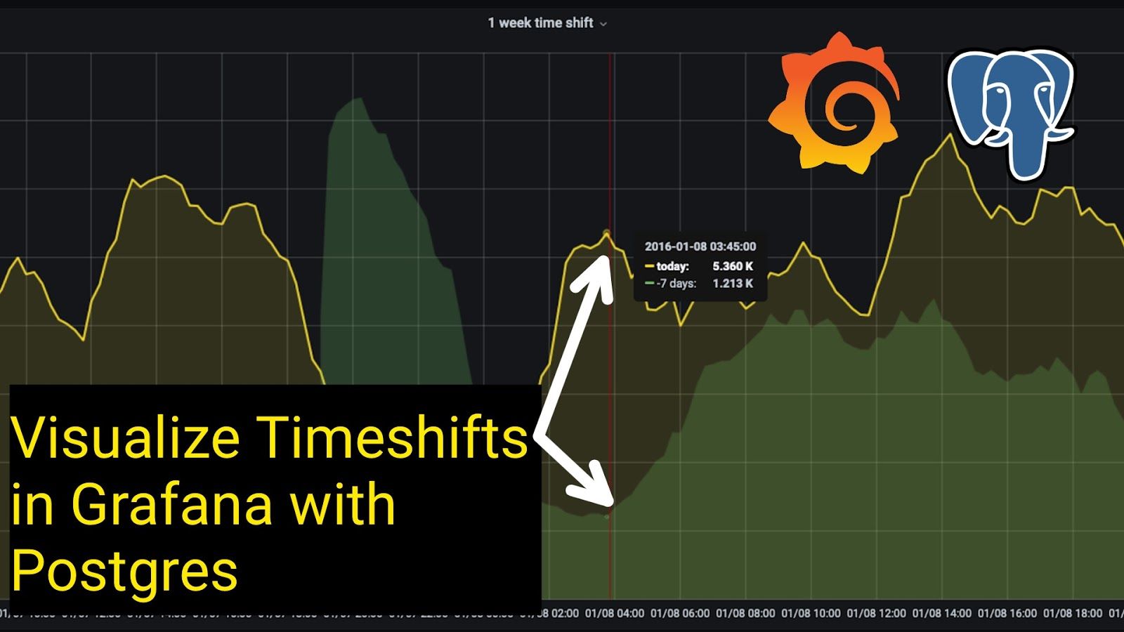
Example 2: Building a 1 Week Timeshifts
Next, we want to answer: “How does the activity this week compare to last week?”
In this example, we create a graph to display the current number of rides, as well as a timeshifted line to graph the rides from the previous week.
Much of the query is the same as in Example 1; the only differences are (1) the interval definition changes from day to week and (2) the series we generate only has two values, 0 and 1, since we only want to compare to the previous week (vs. the 3 day period in the prior example.)
SELECT time, ride_count,
	CASE WHEN step = 0 THEN 'today' ELSE (-interval)::text END AS metric
FROM
    ( SELECT step, (step||'week')::interval AS interval FROM generate_series(0,1) g(step)) g_offsets
JOIN LATERAL (
    SELECT
      time_bucket('15m',pickup_datetime + interval)::timestamptz AS time, count(*) AS ride_count FROM rides
    WHERE
      pickup_datetime BETWEEN $__timeFrom()::timestamptz - interval AND $__timeTo()::timestamptz - interval
    GROUP BY 1
    ORDER BY 1
) l ON trueThis produces the following graph:

Visual Pro-tip: Add a series override
To make it easier to distinguish between rides for any given day and rides from the previous week, we can apply a series override that modifies the appearance of the timeshifted lines:

To achieve this, we set the line area to 0 (under Display settings), and then apply a series override to the timeshifted series.
In the series override settings, we:
- Set the line fill to 2, giving us a shadow look
- Set the line width to 0, leaving the non-timeshifted graph as the only series with a solid line, making it more distinguishable.

Next Steps
In this tutorial, we covered what timeshifting is, how it works, and how to use PostgreSQL LATERAL JOIN, TimescaleDB, and Grafana to visualize timeshifts to easily compare data across two (or more!) time periods.
⏰ To modify the query to timeshift any arbitrary number of minutes, hours, days, months, or years, change the parameters on generate_series and interval definition (while it’s most common to compare metrics NOW to previous periods, you can use time-shifting to compare ANY two time periods).
Happy timeshifting!
Learn More
Want more Grafana tips? Explore our Grafana tutorials (I recommend this one on variables and this one on visualizing missing data).
Need a database to power your dashboarding and data analysis? Get started with Timescale Cloud (it’s our fast, easy-to-use, and reliable cloud-native data platform for time-series, built on PostgreSQL,). When you sign up, you’ll get 30 days of completely free use to get you and up and running.