How to Benchmark IoT Time-Series Workloads in a Production Environment
New IoT dataset available for benchmarking TimescaleDB, MongoDB, InfluxDB, Cassandra & others.
Benchmarking ain’t easy. That is true in general, but can be particularly challenging when comparing the performance of various database technologies for specific workloads. And although it is not the simplest task, it is extremely important to test out these technologies before running them in production scenarios.
Here, our focus is on the IoT industry where we’ve found that many organizations often collect large amounts of time-series data as part of their operations. By collecting data in this way, they are able to conduct real-time and even predictive analysis to better inform current and future decision making.
Now that we understand the value of collecting time-series data, the next logical question becomes: what database should we deploy for an IoT use case? We built a tool to help you answer that question.
Enter the Time Series Benchmark Suite
Last year we announced the availability of the Time Series Benchmark Suite (TSBS) as a tool for comparing and evaluating databases for time-series workloads. The primary goal of TSBS is help take the guesswork out of benchmarking by simplifying the experience of generating time-series datasets, and comparing insert & query performance on a host of database technologies.
Currently TSBS supports TimescaleDB, MongoDB, InfluxDB, Cassandra, ClickHouse, CrateDB and SiriDB. TSBS is designed to be transparent with benchmarking, allowing others to compare and run their own results. (If there’s a technology you’d like to see added, you can submit a GitHub pull request.)
The key with TSBS is that we include specific time-series use cases to bring context to your testing and mimic the workload in a production scenario. We initially released a suite of tests with TSBS that was designed to measure the performance of these database technologies when implemented in the DevOps use case.
Over the past year, we spoke with a number of users who are incorporating time-series workloads into their IoT architecture and the topic of benchmarking was always on the agenda. We took a step back and decided to help users address this topic by expanding the TSBS to include an IoT-specific use case. This use case includes the ability to:
1. Generate data sets that simulate an IoT scenario
2. Benchmark insert/write performance to simulate loading IoT data into database
3. Benchmark query execution performance to simulate analyzing IoT data in the database
In this post, we will share our reasoning behind adding the IoT use case by showcasing how it can be used to simulate an end-to-end real-world IoT scenario. We will also share benchmarking results produced using TSBS for this IoT use case against two popular time-series databases (TimescaleDB and InfluxDB).
If you’ve heard enough and you are interested in trying it out yourself, go straight to the GitHub page. Or see examples of the results TSBS can produce here and here.
Otherwise, please continue reading.
How to generate and load IoT data
As mentioned above, using TSBS for benchmarking involves these phases: generating data sets; benchmarking insert (i.e. “loading”) performance; and benchmarking query (i.e. “analysis”) performance.
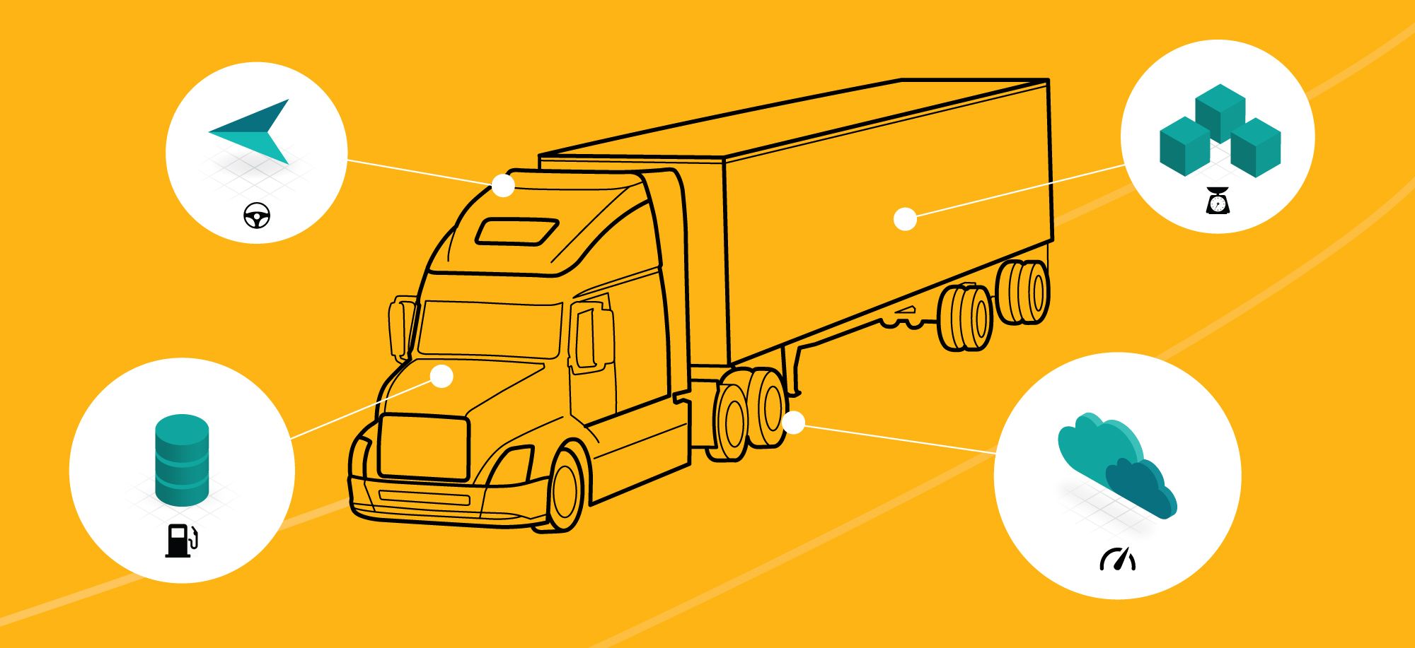
For this new IoT use case, we envisioned these phases playing out based on a fictional trucking company. To demonstrate, we will showcase how to profile data generation by tracking a series of metrics across a fleet of trucks, and offer queries for both real-time analysis of truck activity and predictive analysis for truck maintenance.

In this scenario, there is a device attached to the truck which observes and reports the truck data that we need. The data is a combination of location, diagnostics, and metadata. And as in the real world, data sets are never “perfect” so TSBS also simulates real events that cause the data set to be “less than perfect”.
(LOCATION + DIAGNOSTICS + METADATA) & (REAL EVENTS) = “The IoT Data Set”
Calculating location, diagnostic, and metadata
The location of the truck (as measured by the GPS unit in the form of longitude and latitude of the truck) would be combined with the heading as reported by the sending unit. All of these measurements are reported as individual bits of data on a time interval. This would make up the data that we need to be able to track the truck in real-time (last reported longitude, latitude, and heading). Additionally, we can follow the route of the truck and map all of the historical data points as they relate to positioning and heading from that truck.
(Truck location) metrics we can collect:
- Time
- Longitude
- Latitude
- Elevation
- Velocity
- Heading
- Grade
In addition to collecting (truck location) metrics, we also want to be able to analyze the current conditions (or diagnostics) of the truck as it travels overtime. For example, is the truck low on fuel, or when was the last time the truck stopped for a period of time?
(Truck) diagnostics we can collect:
- Time
- Fuel state
- Fuel consumption
- Current load
- Truck status (moving or stationary)
Next, we would want to introduce (truck) metadata, which allows us to tie our queries to more static assets. For example, what is the average stop time (out of service time) for a given truck model in the fleet? Which drivers obey the speed limits and which present risk? When we start to tie our variable data (metrics) to static metadata, we can start to perform analytics as we roll the data up under these bits of metadata. This is another type of query in the benchmarking stack.
(Truck) metadata we can collect:
- Fleet
- Driver
- Truck model
- Device version
- Load capacity
- Fuel capacity
- Nominal fuel consumption
Simulating real events
Now that we have looked at the data that can be generated, we need to actually create the data sets that also simulate “real world” events that could have an impact on how the system may perform.
Let’s assume that the trucks are transmitting via a wireless network, however, out of network trucks will queue the data locally and when connectivity is established it will push a batch update. We would want to know how this impacts system performance if it happens to a large number of trucks.
The items below represent some of the real events that could impact the system, which we account for in our benchmarking runs.
List of real events that can affect data collection:
- Lots of gaps in the data (representing trucks whose reporting device is broken)
- Out of order ingestion (trucks out of network range, and come back in and report batched data)
- Different versions of input (not all devices on the trucks will run the same firmware)
- Need to correlate data between different time-series
- Often contains geospatial information
How to perform a real-time analysis on the IoT data
From above, we have generated a data set that represents a real IoT use case (and this data set is not “perfect” because we’ve injected real events). Using this data set, we are ready to benchmark insert (“loading”) performance and query (“analysis”) performance. Let's spend some time walking through a preliminary set of benchmark results when we run this against TimescaleDB, a time-series database on PostgreSQL.
Setting up your test platform
We will start by defining the test system. In this case we are running the tests against a system with the following specs:
- 8 CPU
- 30GB RAM
- 1TB Storage (SSD)
In this test we used 2 sets of configurations:
- One set of queries were run 500 times using 8 workers
- Another set of queries was run 100 times using 4 workers
Note: We indicate at the beginning of each result section the frequency and numbers of workers used.
The other set of variables you will need to understand is the size and scale of the data set. In this case we used the following:
- Size of data set: 3 months worth of data (38 million rows) based on data described above
- Scale of data set: 1000 trucks
Note: These parameters are set when you run the script that generates your data, for more information on this, please see the TSBS GitHub repo here.
Measuring ingestion rates
The first measurable statistic we want to look at in our run is how did the database perform during ingestion. Here we are looking at how quickly we were able to take the data from a generated file, introduce our real world scenarios, and see how the database performs.
TimescaleDB ingestion rates (rows per second):

We see that the loading of the dataset, which included variability introduced by the “real world” events we discussed previously, resulted in TimescaleDB loading the generated 38.8 million rows at a rate of 369,141.6 rows per second. This means we were able to load the data set in 105.3 seconds, or in less than 2 minutes.
Another way to look at this (as a way or normalizing results given the different data models used by various time series databases that TSBS supports) is to view at this in terms of number of metrics per second.
TimescaleDB ingestion rates (metrics per second):

When we normalize the data to metrics per second, we see that we are loading 1.8 million metrics per second which gets us to the same total load time. However, we also get a metric to compare against different data models where “rows” is not a relevant concept.
Now that we have looked at some of the basic ingestion numbers and have a good sense for how our database has performed in loading the data, let's take a look at how some of our queries performed.
Testing against sample queries
Before we jump in, we will start with a brief description of each query.

To start producing results, we will walk through a single query and explain how to interpret the results. Next we will broaden the result set so you can see how all of the queries performed.
Let's start by looking at a query we ran that will show us every truck’s last location (our data set here consists of 1,000 trucks).
Total average for a single query in TimescaleDB that we ran 500 times using 8 workers:

Here we queried the database for the last known location of each truck, and on average the database was able to return our result set within 151.64 milliseconds. Given we ran this query 500 times, it is also important to look at the spread of the results. In this case we had a standard deviation of 21.17 ms, meaning on average our results were +/- 21.17 ms from the average query completion time (21.17 ms making up one standard deviation). Expressed another way, our completion time per query was 14% different from the average query completion time. This represents the spread or variability of the results in our run: the higher this number, the more variable our results.
Now that we have walked through the results for a single query, let’s present the rest of results where we run through multiple queries using a larger and smaller configuration.
Multiple queries in TimescaleDB that we ran 500 times using 8 workers:

Multiple queries in TimescaleDB that we ran 100 times using 4 workers:

As you can see, we are presenting the results in such a way that you can get a good sense of what you should expect not just based on TimescaleDB, but also considering the scale of the machine that we have chosen to run on, which will also impact the level of performance. We are also mixing sets of simple and complex queries to complete the profile of what you can expect.
Benchmarks: TimescaleDB vs. InfluxDB
A big part of benchmarking is to have an idea about how your system will perform. The other large piece of benchmarking is trying to perform an “apples-to-apples” comparison of two systems. The above covered how TimescaleDB performed executing an IoT use case. For reference, let's look at a preliminary set of query performance metrics for an alternative time-series database such as InfluxDB.
We start with the same set of data ingestion tests, and measure how InfluxDB performed as it loaded our dataset into the database.
InfluxDB ingestion rates (rows per second):

In this run, we see that the data load took a little more than 3 minutes at 170,045 rows per second. If we want to normalize the data to metrics loaded per second, we can look at the ingestion numbers from that perspective as well.
InfluxDB ingestion rates (metrics per second):

You may notice the difference in the number of metrics. This is one factor that will differ from platform to platform (and why we have a separate data generation process per platform). Here we see that InfluxDB loaded data at a rate of 1.3 million metrics per second.
Next, let’s take a look at how InfluxDB performs using the same queries as the previous test against TimescaleDB.
Multiple queries in InfluxDB that we that we ran 500 times using 8 workers:

Multiple queries in InfluxDB that we ran 100 times using 4 workers:

As you can see, TSBS is able to show us the benchmark results around system performance based on the size and shape of the platform that it is running on (CPU, Memorey, Disk), and the data platform used to run the tests. Here, the common thread is the same data and query patterns based on a real world use case.
In the above, we chose to use TSBS against both TimescaleDB and InfluxDB to run our tests, and were able to produce two independent, but comparable, sets of results.
Comparison of TimescaleDB vs. InfluxDB of the 100 run / 4 worker benchmark results:

Next steps
The idea behind TSBS is to exercise the database in such a way that it will reflect real world IoT use cases of the data and how the database will respond. As a result, we can achieve realistic performance numbers based on a real production workload.
This newly added set of benchmarks are very specific to the IoT use case, and account for the different variables that these workloads encounter in a production environment. The end result allows users to benchmark their system against something that has all of the characteristics of what you will see in production, and really get an understanding of what you can expect in that production environment.
If you are ready to try out TSBS for your IoT use case, visit here for instructions.
Contributions and suggestions
Finally, we’d like to emphasize that TSBS is an open source project, welcoming contributions from the community. If you have feedback for us or ideas around the next set of use cases you would like to see us address, please feel free to swing by the GitHub repo and open an issue with your ideas.
Additionally, if you are interested in benchmarking against databases outside of what is currently supported, your contributions and suggestions are welcome. Simply open an issue, or a pull request via the repository.