How METER Group Brings a Data-Driven Approach to the Cannabis Production Industry

This is an installment of our “Community Member Spotlight” series, where we invite our customers to share their work, shining a light on their success and inspiring others with new ways to use technology to solve problems.

In this edition, Paolo Bergantino, Director of Software for the Horticulture business unit at METER Group, joins us to share how they make data accessible to their customers so that they can maximize their cannabis yield and increase efficiency and consistency between grows.

AROYA is the leading cannabis production platform servicing the U.S. market today. AROYA is part of METER Group, a scientific instrumentation company with 30+ years of expertise in developing sensors for the agriculture and food industries. We have taken this technical expertise and applied it to the cannabis market, developing a platform that allows growers to grow more efficiently and increase their yields – and to do so consistently and at scale.

About the team

My name is Paolo Bergantino. I have about 15 years of experience developing web applications in various stacks, and I have spent the last four here at METER Group. Currently, I am the Director of Software for the Horticulture business unit, which is in charge of the development and infrastructure of the AROYA software platform. My direct team consists of about ten engineers, 3 QA engineers, and a UI/UX Designer. (We’re also hiring!)

About the project

AROYA is built as a React Single-Page App (SPA) that communicates with a Django/DRF back-end. In addition to using Timescale Cloud for our database, we use AWS services such as EC2+ELB for our app and workers, ElastiCache for Redis, S3 for various tasks, AWS IoT/SQS for handling packets from our sensors, and some other services here and there.

✨  Editor’s Note: "Timescale Cloud" is known as "Managed Service for TimescaleDB" as of September 2021.

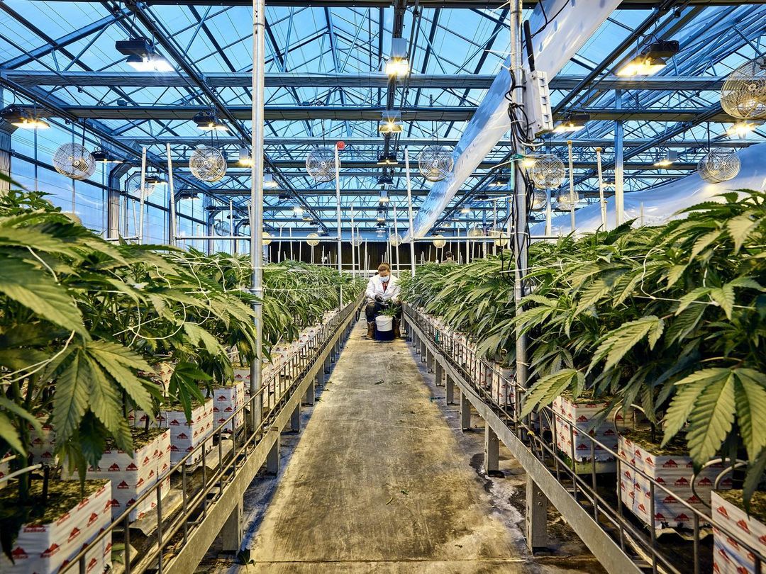
As I previously mentioned, AROYA was born out of our desire to build a system that leveraged our superior sensor technology in an industry that needed such a system. Cannabis worked out great in this respect, as the current legalization movement throughout the U.S. has resulted in a lot of disruption in the space.

The more we spoke to growers, the more we were struck by how much mythology there was in growing cannabis and by how little science was being applied by relatively large operations. As a company with deeply scientific roots, we found it to be a perfect match and an area where we could bring some of our knowledge to the forefront. We ultimately believe the only survivors in the space are those who can use data-driven approaches to their cultivation to maximize their yield and increase efficiency and consistency between grows.

As part of the AROYA platform, we developed a wireless module (called a “nose”) that could be attached to our sensors. Using Bluetooth Low Energy (BLE) for low power consumption and attaching a solar panel to take advantage of the lights in a grow room, the module can run indefinitely without charging.

The most critical sensor we attach to this nose is called the TEROS 12, the three-pronged sensor pictured below. It can be installed into any growing medium (like rockwool, coconut coir, soil, or mixes like perlite, pumice, or peat moss) and give insights into the temperature, water content (WC), and electrical conductivity (EC) of the medium. Without getting too into the weeds (pardon the pun), WC and EC, in particular, are crucial in helping growers make informed irrigation decisions that will steer the plants into the right state and ultimately maximize their yield potential.

We also have an ATMOS 14 sensor for measuring the climate in the rooms and a whole suite of sensors for other use cases.

AROYA’s core competency is collecting this data - e.g., EC, WC, soil temp, air temperature, etc. - and serving it to our clients in real-time (or, at least “real-time” for our purposes, as our typical sampling interval is 3 minutes).

Growers typically split their growing rooms into irrigation zones. We encourage them to install statistically significant amounts of sensors into each room and its zones, so that AROYA gives them good and actionable feedback on the state of their room.  For example, there’s a concept in cultivation called "crop steering" that basically says that if you stress the plant in just the right way,  you can "steer" it into generative or vegetative states at will and drive it to squeeze every last bit of flower. How and when you do this is crucial to doing it properly.

Our data allows growers to dial in their irrigation strategy, so they can hit their target "dryback" for the plant (this is more or less the difference between the water content at the end of irrigation until the next irrigation event). Optimizing dryback is one of the biggest factors in making crop steering work, and it's basically impossible to do well without good data. (We provide lots of other data that helps growers make decisions, but this is one of the most important ones.)

This can be even more important when multiple cultivars (“strains”) of cannabis are grown in the same room, as the differences between two cultivars regarding their needs and expectations can be pretty dramatic. For those unfamiliar with the field, an example might be that different cultivars "drink" water differently, and thus must be irrigated differently to achieve maximum yields. There are also "stretchy" cultivars that grow taller faster than "stocky" ones, and this also affects how they interact with the environment. AROYA not only helps in terms of sensing, but in documenting and helping understand these differences to improve future runs.

The most important thing from collecting all this data is making it accessible to users via graphs and visualizations in an intuitive, reliable, and accurate way, so they can make informed decisions about their cultivation.

We also have alerts and other logic that we apply to incoming data. These visualizations and business logic can happen at the sensor level, at the zone level, at the room level, or sometimes even at the facility level.

A typical use case with AROYA might be that a user logs in to their dashboard to view sensor data for a room. Initially, they view charts aggregated to the zone level, but they may decide to dig deeper into a particular zone and view the individual sensors that make up that zone. Or, vice versa, they may want to pull out and view data averaged all the way up to the room. So, as we designed our solution, we needed to ensure we could get to (and provide) the data at the right aggregation level quickly.

Choosing and using TimescaleDB

The initial solution

During the days of our closed alpha and beta of AROYA with early trial accounts (late 2017 through our official launch December 2019), the amount of data coming into the system was not significant. Our nose was still being developed (and hardware development is nice and slow), so we had to make due with some legacy data loggers that METER also produces. These data loggers only sampled every 5 minutes and, at best, reported every 15 minutes. We used AWS’ RDS Aurora PostgreSQL service and cobbled together a set of triggers and functions that partitioned our main readings table by each client facility – but no more. Because we have so many sensor models and data types we can collect, I chose to use a narrow data model for our main readings table.

This overall setup worked well enough at first, but as we progressed from alpha to beta and our customer base grew, it became increasingly clear that it was not a long-term solution for our time series data needs. I could have expanded my self-managed system of triggers and functions and cobbled together additional partitions within a facility, but this did not seem ideal. There had to be a better way!

I started looking into specific time-series solutions. I am a bit of a home automation aficionado, and I was already familiar with InfluxDB – but I didn’t wish to split my relational data and readings data or teach my team a new query language.

TimescaleDB, being built on top of PostgreSQL, initially drew my attention: it “just worked” in every respect, I could expect it to, and I could use the same tools I was used to for it. At this point, however, I had a few reservations about some non-technical aspects of hosting TimescaleDB that prevented me from going full steam ahead with it.

✨  Editor’s Note: For more comparisons and benchmarks, see how TimescaleDB compares to InfluxDB, MongoDB, AWS Timestream, and other time-series database alternatives on various vectors, from performance and ecosystem to query language and beyond.

Applying a band-aid and setting a goal

Before this point, if I am perfectly truthful, I did not have any serious requirements or standards about what I considered to be the adequate quality of service for our application. I had a bit of an “I know it when I see it” attitude towards the whole thing.

When we had a potential client walk away during a demo due to a particularly slow loading graph, I knew that we had a problem on our hands and that we needed something really solid for the long term.

Still, at the time, we also needed something to get us by until we could perform a thorough evaluation of the available solutions and build something around that. At this point, I decided to stand a Redis cluster between RDS and our application which stored the last 30 days of sensor data (at all the aggregation levels required) as a Pandas dataframe. Any chart request coming in for data within the first 30 days - which accounted for something like 90% of our requests - would simply hit Redis. Anything longer would cobble together the answer using both Redis and querying the database. Performance for the 90% use case was adequate, but it was getting increasingly dreadful as more and more historical data piled up for anything that hit the database.

At this point, I set the goalposts for what our new solution would need to meet: Any chart request, which is an integral part of AROYA, needs to take less than one second for the API to serve.

The research and the first solution

We looked at other databases at this point, InfluxDB was looked at again, we got in a beta of Timestream for AWS and looked at that. We even considered going NoSQL for the whole thing. We ran tests and benchmarks, created matrices of pros and cons, estimated costs, the whole shebang. Nothing compared favorably to what we were able to achieve with TimescaleDB.

Ultimately, the feature that really caught our attention was continuous aggregates in TimescaleDB. The way our logic works, more or less, we see the timeframe that the user is requesting and sample our data accordingly. In other words, if a user fetches three months worth of data, we would not send three months worth of raw data to be graphed to the front-end. Instead, we would bucket our data into appropriately sized buckets that would give us the right amount of data we want to display in the interface.

Although it would require quite a few views, if we created continuous aggregates for every aggregation level and bucket size we cared about, and then directly queried the right aggregation/bucket combination (depending on the parameters requested), that should do it, right? The answer was a resounding yes.

The performance we were able to achieve using these views shattered the competition. Although I admit we were kind of “cheating” by precalculating the data, the point is that we could easily do it. Not only this, but when we ran load tests on our proposed infrastructure, we were blown away by how much more traffic we could support without any service degradation. We could also eliminate all the complicated infrastructure that our Redis layer required, which was quite a load off (literally and figuratively).

The Achilles’ heel of this solution, an astute reader may already notice, is that we were paying for this performance in disk space.

I initially brushed this off as fair trade and moved on with my life. We found TimescaleDB’s compression to be as good as advertised, which gave us 90%+ space savings in our underlying hypertable, but our sizable collection of uncompressed continuous aggregates grew by the day (keep reading to learn why this is a “but”...).

✨ Editor’s Note: We’ve put together resources about continuous aggregates and compression to help you get started.

The “final” solution

AROYA has been on an amazing trajectory since launch, and our growth was evident in the months before and after we deployed our initial TimescaleDB implementation. Thousands upon thousands of sensors hitting the field was great for business – but bad for our disk space.

Our monitoring told a good story of how long our chart requests were taking, as 95%+ of them were under 1 second, and virtually all were under 2 seconds. Still, within a few months of deployment, we needed to upgrade tiers in Timescale Cloud solely to keep up with our disk usage.

✨  Editor’s Note: "Timescale Cloud" is known as "Managed Service for TimescaleDB" as of September 2021.

We had adequate computing resources for our load, but 1 TB was no longer enough, so we doubled our total instance size to get another 1 TB. While everything was running smoothly, I felt a dark cloud overhead as our continuous aggregates grew and grew in size.

The clock was ticking, and before we knew it, we were coming up on 2 TB of readings. So, we had to take action.

We had attended a webinar hosted by Timescale and heard someone make a relatively off-hand comment about rolling their own compression for continuous aggregates. This planted a seed that was all we needed to get going.

The plan was thus: first, after consulting with Timescale staff, we were alerted we had way too many bucket sizes. We could use TimescaleDB’s time_bucket functions to do some of this on the fly without affecting performance or keeping as many continuous aggregates. That was an easy win.

Next, we split each of our current continuous aggregates into three separate components:

• First, we kept the original continuous aggregate.
• Then, we leveraged the TimescaleDB job scheduler to move and compress chunks from the original continuous aggregate into a hypertable for that specific bucket/aggregation view.
• Finally, we created a plain old view that UNIONed the two and made it a transparent change for our application.

This allowed us to compress everything but the last week of all of our continuous aggregates, and the results were as good as we could have hoped for.

We were able to take our ~1.83 TB database and compress it down to 700 GB. Not only that, about 300 GB of that is log data that’s unrelated to our main reading pipeline.

We will be migrating out this data soon, which gives us a vast amount of room to grow. (We think we can even move back the 1TB plan at this point, but have to test to ensure that compute doesn’t become an issue.) The rate of incrementation in disk usage was also massively slowed, which bodes well for this solution in the long term. What’s more, there was virtually no penalty for doing this in terms of performance for any of the metrics we monitor.

Ultimately TimescaleDB had wins across the board for my team. Performance was going to be the driving force behind whatever we went with, and TimescaleDB has delivered that in spades.

Current deployment & future plans

We currently ingest billions of readings every month using TimescaleDB and couldn’t be happier. Our data ingest and charting capabilities are two of the essential aspects of AROYA’s infrastructure.

While the road to get here has been a huge learning experience, our current infrastructure is straightforward and performant, and we’ve been able to rely on it to work as expected and to do the right thing. I am not sure I can pay a bigger compliment than that.

We’ve recently gone live with our AROYA Analytics release, which is building upon what we’ve done to deliver deeper insights into the environment and the operations at the facilities using our service. Every step of the way, it’s been straightforward (and performant!) to calculate the metrics we need with our TimescaleDB setup.

Getting started advice & resources

I think it’s worth mentioning that there were many trade-offs and requirements that guided me to where AROYA is today with our use of TimescaleDB. Ultimately, my story is simply the set of decisions that led me to where we are now and people’s mileage may vary depending on their requirements.

I am sure that the set of functionality offered means that, with a little bit of creativity, TimescaleDB can work for just about any time-series use case I can think of.

The exercise we went through when iterating from our initial non-Timescale solution to Timescale was crucial to get me to be comfortable with that migration. Moving such a critical part of my infrastructure was scary, and it is still scary.

Monitoring everything you can, having redundancies, and being vigilant about any unexpected activity - even if it’s not something that may trigger an error - has helped us stay out of trouble.

We have a big Grafana dashboard on a TV in our office that displays various metrics and multiple times we’ve seen something odd and uncovered an issue that could have festered into something much more if we hadn’t dug into it right away. Finally, diligent load testing of the infrastructure and staging runs of any significant modifications have made our deployments a lot less stressful, since they instill quite a bit of confidence.

✨ Editor’s Note: Check out Grafana 101 video series and Grafana tutorials to learn everything from building awesome, interactive visualizations to setting up custom alerts, sharing dashboards with teammates, and solving common issues.

I would like to give a big shout-out to Neil Parker, who is my right-hand man in anything relating to AROYA infrastructure and did virtually all of the actual work in getting many of these things set up and running. I would also like to thank Mike Freedman and Priscila Fletcher from Timescale, who have given us a great bit of time and information and helped us in our journey with TimescaleDB.

We’d like to give a big thank you to Paolo and everyone at AROYA for sharing their story, as well as for their efforts to help transform the cannabis production industry, equipping growers with the data they need to improve their crops, make informed decisions, and beyond.

We’re always keen to feature new community projects and stories on our blog. If you have a story or project you’d like to share, reach out on Slack (@Lucie Šimečková), and we’ll go from there.

Additionally, if you’re looking for more ways to get involved and show your expertise, check out the Timescale Heroes program.