Charting the Spread of COVID-19 Using Data
Data gives us insight into the world around us – and allows us to visualize and prepare for the spread of the COVID-19 pandemic.
In recent months, we’ve seen the spread of the COVID-19 virus (commonly referred to as "coronavirus"). Not only are we a globally distributed team, some Timescale team family members see fears and concerns first-hand while working in our emergency rooms.
First and foremost, our thoughts are with those who've been affected in any way. We join the global community in hoping for the best in the coming weeks and months, especially in containing transmission and reducing the virus' spread.
We were recently made aware of a time-series dataset from Johns Hopkins University, containing daily case reports from around the world. Timescale community member Joel Natividad created this repo of time-series utilities that enables people to use the Johns Hopkins University dataset with TimescaleDB to better monitor the COVID-19 situation.
In this post, we'll walkthrough how to load the dataset into TimescaleDB and use Grafana to visualize queries. Our hope is that you’ll be able to use this dataset and tutorial as a starting point for your own analysis (extending upon the queries we include), or to share information with colleagues, family, and friends.
You can get TimescaleDB in two forms: Managed Service for TimescaleDB (with free credits) or TimescaleDB for download. You can follow these instructions to choose your installation method. If you haven’t done so, you’ll also want to install psql to access the database from your command line.
Ingesting the dataset
Once you’ve installed TimescaleDB, you will need to load the dataset. First, you will want to clone the GitHub repository Joel created:
git clone https://github.com/dathere/covid19-time-series-utilities.gitThis repository contains several files, which are explained in the README. Setup your database and ingest the data according to the instructions in the GitHub repository.
Once the data is fully ingested, you should be able to login to your database from psql:
psql -x "postgres://[YOUR USERNAME]:[YOUR PASSWORD]@[YOUR HOST]:[YOUR PORT]/[DB_NAME]?sslmode=require"Once you’re logged in, you will be able to run the following query:
SELECT * FROM covid19_ts LIMIT 5;Your output should look something like this:
province_state | country_region |    observation_date    | confirmed | deaths | recovered
---------------+----------------+------------------------+-----------+--------+-----------
Hubei          | Mainland China | 2020-01-31 23:59:00+00 |      5806 |    204 |       141
Zhejiang       | Mainland China | 2020-01-31 23:59:00+00 |       538 | [null] |        14
Guangdong      | Mainland China | 2020-01-31 23:59:00+00 |       436 | [null] |        11
Henan          | Mainland China | 2020-01-31 23:59:00+00 |       352 |      2 |         3
Hunan          | Mainland China | 2020-01-31 23:59:00+00 |       332 | [null] |         2
(5 rows)
At this point, your time-series database is properly configured and you've loaded the COVID-19 dataset.
Note: the Johns Hopkins University data is a running total, not a per-day total. So, the data for February 23rd for any given location represents a cumulative tally of all cases in that location as of February 23rd.
Before we continue, we need to clean up our dataset.
In some cases, a given row in the covid19_ts or covid19_locations table may not have a province_state entered properly. Cleaning public datasets is fairly common, and fortunately, this dataset is easy to prepare for the rest of our tutorial. In psql enter the following commands:
UPDATE covid19_locations
SET province_state =
    CASE WHEN province_state = ''
    THEN country_region
    ELSE province_state
    END;
At this point, all our rows have either a specific Province or State in the province_state column, or, failing that, we default to the country_region.
Now, let’s start running queries that will give us some insight into the pandemic.
How many confirmed cases were reported worldwide each day?
Let’s start by identifying how many cumulative cases have been identified each day; the dataset starts on January 22nd, so that’s where we'll start for our query.
SELECT time_bucket('1 day', observation_date) AS day,
       SUM(confirmed)
FROM covid19_ts
GROUP BY day
ORDER BY day;
Your output should look something like this:
         day           |  sum
-----------------------+-------
2020-01-22 00:00:00+00 |   555
2020-01-23 00:00:00+00 |   653
2020-01-24 00:00:00+00 |   941
2020-01-25 00:00:00+00 |  1438
2020-01-26 00:00:00+00 |  2118
2020-01-27 00:00:00+00 |  2927
2020-01-28 00:00:00+00 |  5578
2020-01-29 00:00:00+00 |  6165
2020-01-30 00:00:00+00 |  8235
2020-01-31 00:00:00+00 | 10037
2020-02-01 00:00:00+00 | 12009
2020-02-02 00:00:00+00 | 16685
2020-02-03 00:00:00+00 | 19719
2020-02-04 00:00:00+00 | 23821
2020-02-05 00:00:00+00 | 27457
(edited for length)
How many confirmed cases have been reported each day near Milan, Italy?
As of the publication date of this post, northern Italy has the highest concentration of COVID-19 cases, outside of China, and it continues to intensify.
What if we wanted to see the growth rate of COVID-19 in Italy?
To do this, we query on the country_region field in our database:
SELECT * FROM covid19_ts WHERE country_region = 'Italy';Our output will look something like this:
province_state | country_region | observation_date       | confirmed | deaths | recovered
---------------+----------------+------------------------+-----------+--------+-----------
               | Italy          | 2020-01-31 23:59:00+00 |         2 | [null] |    [null]
               | Italy          | 2020-01-31 08:15:00+00 |         2 |      0 |         0
               | Italy          | 2020-01-31 08:15:53+00 |         2 |      0 |         0
               | Italy          | 2020-02-07 17:53:02+00 |         3 |      0 |         0
               | Italy          | 2020-02-21 23:33:06+00 |        20 |      1 |         0
               | Italy          | 2020-02-22 23:43:02+00 |        62 |      2 |         1
               | Italy          | 2020-02-23 23:43:02+00 |       155 |      3 |         2
               | Italy          | 2020-02-24 23:43:01+00 |       229 |      7 |         1
               | Italy          | 2020-02-25 18:55:32+00 |       322 |     10 |         1
               | Italy          | 2020-02-26 23:43:03+00 |       453 |     12 |         3
               | Italy          | 2020-02-27 23:23:02+00 |       655 |     17 |        45
               | Italy          | 2020-02-28 20:13:09+00 |       888 |     21 |        46
               | Italy          | 2020-02-29 18:03:05+00 |      1128 |     29 |        46
               | Italy          | 2020-03-01 23:23:02+00 |      1694 |     34 |        83
               | Italy          | 2020-03-02 20:23:16+00 |      2036 |     52 |       149
(15 rows)
How many confirmed cases have been reported each week near me?
What if we wanted to look at cases near a specific location?
This requires that we make use of the latitude and longitude information stored in our database. To use the location, we’ll need to get our tables ready for geospatial queries.
One caveat: The Johns Hopkins University dataset has limited information about specific locations. All cases in Italy are marked as “Italy,” for example, while cases in China and the United States may be more specific with regional or city locations.
We can use the PostGIS PostgreSQL extension to help analyze geospatial data. (This is available out-of-the-box on Managed Service for TimescaleDB, or you can manually install for self-hosted versions.) PostGIS allows us to slice data by time and location within TimescaleDB.
CREATE EXTENSION postgis;Then, run the \dx command in psql to verify that PostGIS was installed properly. You should see the PostGIS extension in your extension list, as noted below:
List of installed extensions
Name        | Version |   Schema   |                             Description
------------+---------+------------+---------------------------------------------------------------------
plpgsql     | 1.0     | pg_catalog | PL/pgSQL procedural language
postgis     | 2.5.3   | public     | PostGIS geometry, geography, and raster spatial types and functions
timescaledb | 1.6.0   | public     | Enables scalable inserts and complex queries for time-series data
(3 rows)
The covid19_locations table in our database includes the locations in the Johns Hopkins University dataset, as well as their latitude and longitude coordinates.
For example, we can see all the locations in the United States like so:
SELECT * FROM covid19_locations WHERE country_region = 'US' LIMIT 10;The output for this query looks something like this:
               province_state                | country_region | latitude | longitude
---------------------------------------------+----------------+----------+-----------
 Unassigned Location (From Diamond Princess) | US             |  35.4437 |  139.6380
 King County, WA                             | US             |  47.5480 | -121.9836
 Santa Clara, CA                             | US             |  37.3541 | -121.9552
 Snohomish County, WA                        | US             |  48.0330 | -121.8339
 Cook County, IL                             | US             |  41.7377 |  -87.6976
 Fulton County, GA                           | US             |  33.8034 |  -84.3963
 Grafton County, NH                          | US             |  43.9088 |  -71.8260
 Hillsborough, FL                            | US             |  27.9904 |  -82.3018
 Providence, RI                              | US             |  41.8240 |  -71.4128
 Sacramento County, CA                       | US             |  38.4747 | -121.3542
(10 rows)
We need to alter the covid19_locations table to work with PostGIS.
To start, we’ll add geometry columns for case locations:
ALTER TABLE covid19_locations
    ADD COLUMN location_geom geometry(POINT, 2163);
Next we’ll need to convert the latitude and longitude points into geometry coordinates (so they play well with PostGIS).
UPDATE covid19_locations
    SET location_geom = ST_Transform(ST_SetSRID(ST_MakePoint(longitude, latitude), 4326), 2163);
Lastly, let’s say we want to examine cases near Seattle, in the United States. Seattle is located at (lat, long) (47.6062,-122.3321).
Our database is setup, so we're ready to run a geospatial query that returns the number of confirmed COVID-19 cases within 75km of Seattle, each day, since the start of our dataset. (TimescaleDB is based on PostgreSQL, so we can use all our favorite SQL functions.)
In this case, we need to use a subquery for the information in our covid19_locations table and a broader query for all confirmed cases that match the locations in our subquery.
First, we write the subquery by querying the covid19_locations table for all locations within 75km of Seattle:
SELECT *
FROM covid19_locations
WHERE ST_Distance(location_geom, ST_Transform(ST_SetSRID(ST_MakePoint(-122.3321, 47.6062), 4326), 2163)) < 75000;
We should get output that looks like this:
province_state       | country_region | latitude | longitude |                   location_geom
---------------------+----------------+----------+-----------+----------------------------------------------------
King County, WA      | US             |  47.5480 | -121.9836 | 010100002073080000A2B8C609FEC838C1004A6D25430F1F41
Snohomish County, WA | US             |  48.0330 | -121.8339 | 010100002073080000344A7104C26438C1768752D481082141
(2 rows)
Now, we need to find all confirmed cases in our covid19_ts dataset whose province_state matches the result of our first query.
SELECT time_bucket('1 day', observation_date) as day,
       SUM(confirmed) AS near_sea
FROM covid19_ts
WHERE province_state IN (
    SELECT province_state
    FROM covid19_locations
    WHERE ST_Distance(location_geom, ST_Transform(ST_SetSRID(ST_MakePoint(-122.3321, 47.6062), 4326), 2163)) < 75000
)
GROUP BY day
ORDER BY day;
Your output should look something like this:
          day           | near_sea
------------------------+----------
 2020-02-29 00:00:00+00 |        1
 2020-03-01 00:00:00+00 |        2
 2020-03-02 00:00:00+00 |       18
 2020-03-03 00:00:00+00 |       27
 2020-03-04 00:00:00+00 |       39
(5 rows)
Use Grafana to visualize confirmed cases by geographic location
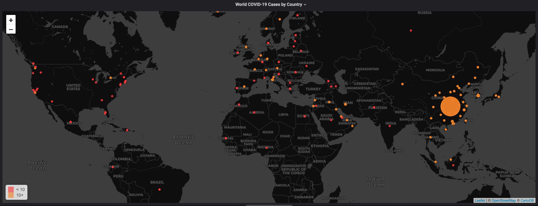
We have the dataset, we have our queries, and, now, let's take the COVID-19 dataset and visualize the total number of confirmed cases by geographic location.
To create our visualization, we’ll use Grafana. Follow our short tutorial on getting started with Grafana to setup Grafana in Managed Service for TimescaleDB, your desktop, or using Grafana Cloud, using the dataset you’ve been using in this post.
In Grafana, create a new dashboard and add a new visualization. In the visualization menu, search for and select the WorldMap panel type.
To build our visualization, we will need our information organized properly in our query:
- For each day
- A sum of all confirmed cases
- Grouped by the
province_statewhere they happened - Plotted on the map using the latitude and longitude for the
province_state - Ordered by time
To build this query, we use a SQL INNER JOIN statement to combine information from the covid19_ts dataset and the covid19_locations tables:
SELECT time_bucket('1 day', covid19_ts.observation_date) AS day,
       SUM(covid19_ts.confirmed) AS confirmed,
       covid19_ts.province_state as location,
       covid19_locations.latitude AS latitude,
       covid19_locations.longitude AS longitude
FROM covid19_ts
INNER JOIN covid19_locations ON covid19_locations.province_state = covid19_ts.province_state
WHERE $__timeFilter(covid19_ts.observation_date)
GROUP BY day,
         confirmed,
         location,
         latitude,
         longitude
ORDER BY day;
To enter this query in Grafana, click “Edit SQL” and type it in manually (or copy-paste from the above):

And then in the WorldMap configuration, we set the field mapping to match our query results:

And, once completed, we see the impact of the COVID-19 pandemic on the Grafana WorldMap panel:

How rapidly is COVID-19 spreading near me?
As mentioned earlier, the Johns Hopkins dataset includes cumulative data. For example, an entry for March 2, 2020 contains all cases that have been confirmed at that point in time. Suppose we wanted to learn the rate at which cases have been identified near a specific location.
TimescaleDB includes a feature called continuous aggregates. A continuous aggregate recomputes a query automatically at user-specified time intervals and maintains the results into a table. Thus, instead of everyone running an aggregation query each time, the database can run a common aggregation periodically in the background, and users can query the results of the aggregation. Continuous aggregates should improve database performance and query speed for common calculations.
In our case, we want to maintain a continuous aggregation for the daily change in confirmed cases. Let's look at this continuous aggregation query:
CREATE VIEW daily_change
WITH (timescaledb.continuous, timescaledb.refresh_lag = '-2 days')
AS
SELECT
  country_region,
  province_state,
  time_bucket('2 days', observation_date) as bucket,
  first(confirmed, observation_date) as yesterday,
  last(confirmed, observation_date) as today,
  last(confirmed, observation_date) - first(confirmed, observation_date) as change
FROM
  covid19_ts
GROUP BY country_region, province_state, bucket;
The first line of this query creates a continuous aggregation named daily_change. We then select a time_bucket with an interval of two days calculated using the covid19_ts.observation_date field.
In our table, we'll create a yesterday and today column, as well as a change column that represents the delta between the two.
Under normal circumstances with large amounts of data, TimescaleDB calculates continuous aggregates in the background, but if you want to see the result immediately, you can force it:
ALTER VIEW daily_change SET (timescaledb.refresh_interval = '1 hour');
ALTER VIEW daily_change SET (timescaledb.refresh_lag = '-2 days');
REFRESH MATERIALIZED VIEW daily_change;
We can run this continuous aggregation with a simple SQL query:
SELECT * FROM daily_change;The result of that query should look something like this:
          day           | yesterday | today  | change |                  location
------------------------+-----------+--------+--------+---------------------------------------------
 2020-01-22 00:00:00+00 |         2 | [null] | [null] |
 2020-01-22 00:00:00+00 |         1 |      9 |      8 | Anhui
 2020-01-22 00:00:00+00 |    [null] | [null] | [null] | Australia
 2020-01-22 00:00:00+00 |        14 |     22 |      8 | Beijing
 2020-01-22 00:00:00+00 |    [null] | [null] | [null] | Brazil
 2020-01-22 00:00:00+00 |         6 |      9 |      3 | Chongqing
 2020-01-22 00:00:00+00 |    [null] | [null] | [null] | Colombia
 2020-01-22 00:00:00+00 |         1 |      5 |      4 | Fujian
 2020-01-22 00:00:00+00 |    [null] |      2 | [null] | Gansu
 2020-01-22 00:00:00+00 |        26 |     32 |      6 | Guangdong
We can also incorporate the continuous aggregation in other queries, such as the one we used earlier to see the rate of change in confirmed cases near Seattle, Washington.
SELECT bucket,
       yesterday,
       today,
       change,
       province_state,
       country_region
FROM daily_change
WHERE province_state IN (
    SELECT province_state
    FROM covid19_locations
    WHERE ST_Distance(location_geom, ST_Transform(ST_SetSRID(ST_MakePoint(-122.3321, 47.6062), 4326), 2163)) < 75000
)
GROUP BY bucket,
         yesterday,
         today,
         change,
         province_state,
         country_region
ORDER BY bucket;
Our output should look like this:
         bucket         | yesterday | today | change |    province_state    | country_region
------------------------+-----------+-------+--------+----------------------+----------------
 2020-02-29 00:00:00+00 |         1 |     2 |      1 | Snohomish County, WA | US
 2020-03-02 00:00:00+00 |         4 |     6 |      2 | Snohomish County, WA | US
 2020-03-02 00:00:00+00 |        14 |    21 |      7 | King County, WA      | US
 2020-03-04 00:00:00+00 |         8 |     8 |      0 | Snohomish County, WA | US
 2020-03-04 00:00:00+00 |        31 |    31 |      0 | King County, WA      | US
(5 rows)
Conclusion
Data gives us insight into the world around us and understanding data enables us to communicate these insights to many people. We encourage you to explore the dataset and share your dashboards and insights on Twitter using #Covid19Data (@-mention @TimescaleDB if you have questions or comments).
If you need help using TimescaleDB or writing visualizations of your own, follow the Hello, Timescale! tutorial. And, join our Slack to ask questions and get help from the global community of Timescale users (our engineering team is also active on all channels).
Finally, no matter where you are, take prudent actions to prepare yourself and your family. Please follow the guidelines and instructions from the World Health Organization.