Best Practices for Query Optimization on PostgreSQL

The demands of modern applications and the exponential growth of data in today’s data-driven world have put immense pressure on databases. Traditional relational databases, including PostgreSQL, are increasingly being pushed to their limits as they struggle to cope with the sheer scale of data that needs to be processed and analyzed, requiring constant query optimization practices and performance tweaks.
Having built our product on PostgreSQL, at Timescale we’ve written extensively on the topic of tweaking your PostgreSQL database performance, from how to size your database, key PostgreSQL parameters, database indexes, and designing your schema to PostgreSQL partitioning.
In this article, we aim to explore best practices for enhancing query optimization in PostgreSQL. We’ll offer insights into optimizing queries, the importance of indexing, data type selection, and the implications of fluctuating data volumes and high transaction rates.
Let’s jump right in.
Why Is PostgreSQL Query Optimization Necessary?
Optimizing your PostgreSQL queries becomes a necessity when performance issues significantly impact the efficiency and functionality of your PostgreSQL database, making your application sluggish and impacting the user experience. Before we dive into the solutions, let’s look at some of the key contributors to performance issues in PostgreSQL:
Inefficient queries: The impact of poorly optimized or complex queries on PostgreSQL's performance is profound. These queries act as significant bottlenecks, impeding data processing efficiency and overall database throughput. Regular analysis and refinement of these query structures are not just beneficial but crucial for maintaining optimal database performance. Understanding and optimizing SQL queries is essential for efficient database operations. This knowledge is pivotal for developing efficient and responsive database operations, ensuring the database's capability to handle complex data workloads effectively.
Insufficient indexes: Inadequate indexing can significantly slow down query execution in PostgreSQL. Strategically implementing indexes, particularly on columns that are frequently accessed, can drastically enhance performance and optimize database responsiveness. Effective indexing strategies are not only crucial for accelerating query speeds but also play a main role in optimizing the efficiency of complex queries and large-scale data operations, ensuring a more responsive and robust database environment.
Over-indexing: While it's true that insufficient indexing can hurt your PostgreSQL performance, it's equally important not to overdo it. Excessive indexes can lead to their own set of challenges: each additional index introduces overhead during your INSERTs, UPDATEs, and DELETEs, they consume disk space and can make database maintenance tasks (such as vacuuming) more time-consuming.
Inappropriate data types: Using unsuitable data types in PostgreSQL can lead to increased storage usage and slower query execution, as inappropriate types may need additional processing and can occupy more storage space than necessary. Carefully selecting and optimizing data types to align with the specific characteristics of the data is a critical aspect of database optimization. The right choice of data types not only influences overall database performance but also contributes to storage efficiency. Additionally, it helps in avoiding costly type conversions during database operations, thereby streamlining data processing and retrieval.
Fluctuating data volume: PostgreSQL's query planner relies on up-to-date data statistics to formulate efficient execution plans. Fluctuations in data volume can significantly impact these plans, potentially leading to suboptimal performance if the planner operates on outdated information. As data volumes change, it becomes crucial to regularly assess and adapt execution plans to these new conditions. Keeping the database statistics current is essential, as it enables the query planner to accurately assess the data landscape and make informed decisions, thereby optimizing query performance and ensuring the database responds effectively to varying data loads.
High transaction volumes: Large numbers of transactions can significantly strain PostgreSQL's resources, especially in high-traffic or data-intensive environments. Effectively leveraging read replicas in PostgreSQL can substantially mitigate the impact of high transaction volumes, ensuring a more efficient and robust database environment.
Hardware limitations: Constraints in CPU, memory, or storage can create significant bottlenecks in PostgreSQL's performance, as these hardware limitations directly affect the database's ability to process queries, handle concurrent operations, and store data efficiently. Upgrading hardware components, such as increasing CPU speed, expanding memory capacity, or adding more storage, can provide immediate improvements in performance. Additionally, optimizing resource allocation, like adjusting memory distribution for different database processes or balancing load across storage devices, can also effectively alleviate these hardware limitations.
Lock contention: Excessive locking on tables or rows in PostgreSQL, particularly in environments that handle parallel queries, can lead to significant slowdowns, inconsistent data, and locking issues. This is because row-level or table-level locks can restrict data access, leading to increased waiting times for other operations and potentially causing queuing delays. Therefore, judicious use of locks is crucial in maintaining database concurrency and ensuring smooth operation. Strategies such as using less restrictive lock types, designing transactions to minimize locked periods, and optimizing query execution plans can help reduce lock contention.
Lack of maintenance: Routine maintenance tasks such as vacuuming, reindexing, and updating statistics are fundamental to sustaining optimal performance in PostgreSQL databases. Vacuuming is essential for reclaiming storage space and preventing transaction ID wraparound issues, ensuring the database remains efficient and responsive. Regular reindexing is crucial for maintaining the speed and efficiency of index-based query operations, as indexes can become fragmented over time. Additionally, keeping statistics up-to-date is vital for the query planner to make well-informed decisions, as outdated statistics can lead to suboptimal query plans. Ignoring these tasks can lead to a gradual but significant deterioration in database efficiency and reliability.
How to Measure Query Performance in PostgreSQL
pg_stat_statements
To optimize your queries, you must first identify your PostgreSQL performance bottlenecks. A simple way to do this is using pg_stat_statements, a PostgreSQL extension that provides essential information about query performance. It records data about running queries, helping to identify performance slowdowns caused by inefficient queries, index changes, or ORM query generators. Notably, pg_stat_statements is enabled by default in TimescaleDB, enhancing its capability to monitor and optimize database performance out of the box.
You can query pg_stat_statements to gather various statistics such as the number of times a query has been called, total execution time, rows retrieved, and cache hit ratios:
-
Identifying long-running queries: Focus on queries with high average total times, adjusting the
callsvalue based on specific application needs. -
Hit cache ratio: This metric measures how often data needed for a query was available in memory, which can affect query performance.
-
Standard deviation in query execution time: Analyzing the standard deviation can reveal the consistency of query execution times, helping to identify queries with significant performance variability.
Insights by Timescale
Timescale’s Insights (available to Timescale users at no extra cost) is a tool providing in-depth observation of PostgreSQL queries over time. It offers detailed statistics on query timing, latency, and memory and storage I/O usage, enabling users to comprehensively monitor and analyze their query and database performance.
-
Scalable query collection system: Insights is built on a scalable system that collects sanitized statistics on every query stored in Timescale, facilitating comprehensive analysis and optimization. And the best part is that the team is dogfooding its own product to enable this tool, expanding PostgreSQL to accommodate hundreds of TBs of data (and growing).
-
Insights interface: The tool presents a graph showing the relationship between system resources (CPU, memory, disk I/O) and query latency.
-
Detailed query information: Insights provides a table of the top 50 queries based on chosen criteria, offering insights into query frequency, affected rows, and usage of Timescale features like hypertables and continuous aggregates.
-
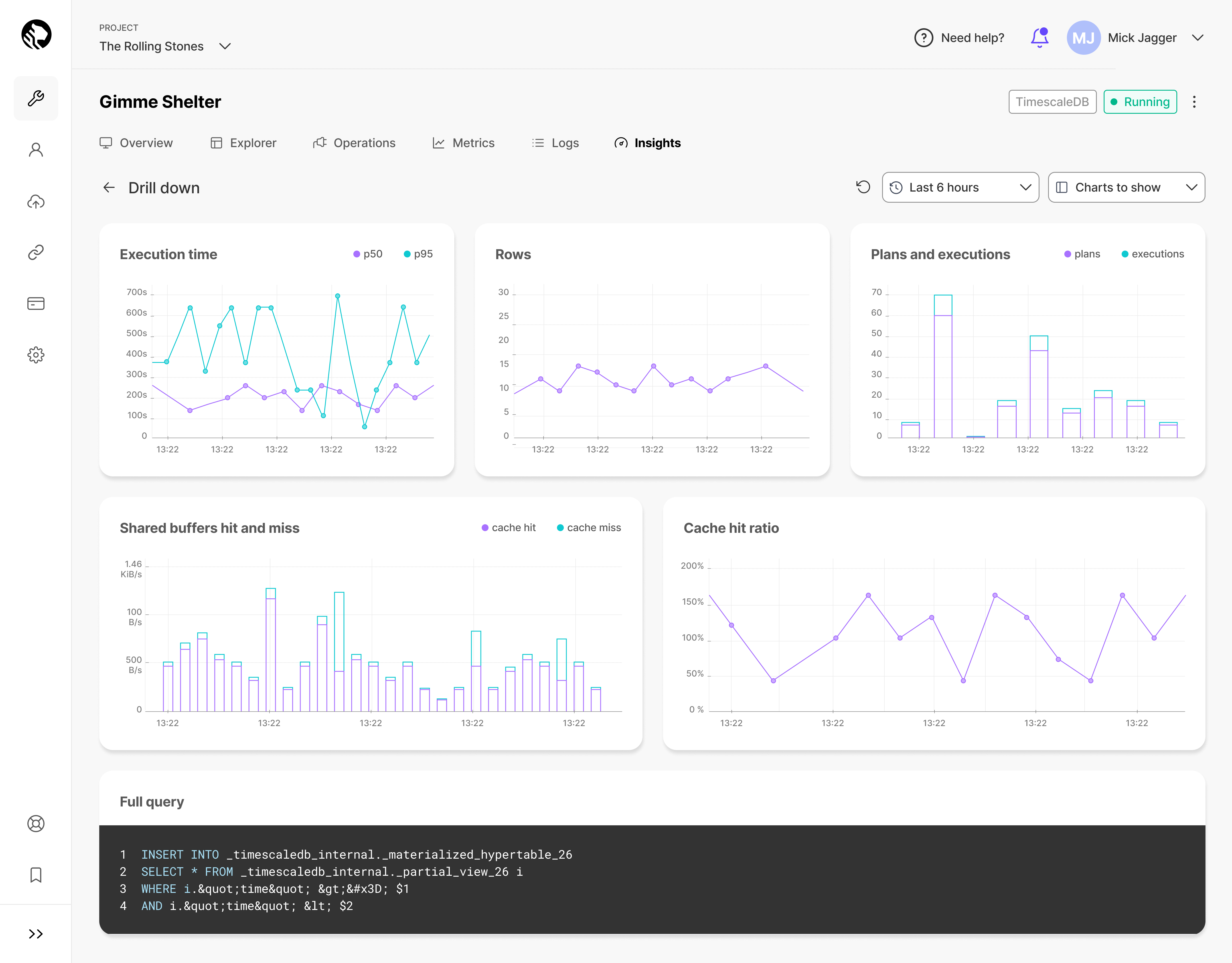
Drill-down view: Insights offers a drill-down view with finer-grain metrics, including trends in latency, buffer usage, and cache utilization.
-
Real-world application: Check out the Humblytics story, which demonstrates Insights' practical application in identifying and resolving performance issues.
Best Practices for Query Optimization in PostgreSQL
Understand common performance bottlenecks
To effectively identify inefficient queries so you can optimize them, analyze query execution plans using PostgreSQL's EXPLAIN command. This tool provides a breakdown of how your queries are executed, revealing critical details such as execution paths and the use of indexes. Look specifically for patterns like full table scans, which suggest missing indexes or queries consuming high CPU or memory, indicating potential optimizations. By understanding the intricacies of the execution plan, you can pinpoint exactly where performance issues are occurring.
For example, you could run the following code to view the execution plan of a query:
EXPLAIN SELECT * FROM your_table WHERE your_column = 'value';
To identify full table scans, you would look for “Seq Scan” in the output. This suggests that the query is scanning the entire table, which is often a sign that an index is missing or not being used effectively:
Seq Scan on large_table (cost=0.00..1445.00 rows=50000 width=1024)
Partition your data
Partitioning large PostgreSQL tables is a powerful strategy to enhance their speed and efficiency. However, the process of setting up and maintaining partitioned tables can be burdensome, often requiring countless hours of manual configurations, testing, and maintenance. But, there's a more efficient solution: hypertables. Available through the TimescaleDB extension and on AWS via the Timescale platform, hypertables simplify the PostgreSQL partition creation process significantly by automating the generation and management of data partitions without altering your user experience. Behind the scenes, however, hypertables work their magic, accelerating your queries and ingest operations.
To create a hypertable, create a regular PostgreSQL table:
CREATE TABLE conditions (
   time        TIMESTAMPTZ       NOT NULL,
   location    TEXT              NOT NULL,
   device      TEXT              NOT NULL,
   temperature DOUBLE PRECISION  NULL,
   humidity    DOUBLE PRECISION  NULL
);
Then, convert the table to a hypertable. Specify the name of the table you want to convert and the column that holds its time values.
SELECT create_hypertable('conditions', by_range('time'));
Employ partial aggregation for complex queries
Continuous aggregates in TimescaleDB are a powerful tool to improve the performance of commonly accessed aggregate queries over large volumes. Continuous aggregates are based on PostgreSQL materialized views but incorporate incremental and automatic refreshes so they are always up-to-date and remain performant as the underlying dataset grows.
In the example below, we’re setting up a continuous aggregate for daily average temperatures, which is remarkably simple.
CREATE VIEW daily_temp_avg
WITH (timescaledb.continuous)
AS
SELECT time_bucket('1 day', time) as bucket, AVG(temperature)
FROM hypertable
GROUP BY bucket;
Learn how continuous aggregates can help you get real-time analytics or create a time-series graph.
Continuously update and educate
Regularly updating PostgreSQL and TimescaleDB is vital for performance and security. The upgrade process involves assessing changes, performance gains, security patches, and extension compatibility. Focus on best practices, which include upgrading major versions at minor version .2 for stability, consistently updating minor versions, and upgrading major versions when needed for functionality or security. Timescale further eases this process by handling minor updates automatically with no downtime and providing tools for testing major version upgrades, ensuring smooth transitions with minimal disruption.
Conclusion
Optimizing your queries in PostgreSQL doesn’t have to be a daunting task. While it involves understanding and addressing various factors, there is much you can do by adopting best practices, such as efficient indexing, judicious use of data types, regular database maintenance, and staying up-to-date with the latest PostgreSQL releases.
If you really want to extend PostgreSQL’s capabilities, create a free Timescale account today. Features such as hypertables, continuous aggregates, and advanced data management techniques significantly enhance PostgreSQL's ability to manage your demanding workloads effectively.
Written by Paulinho Giovannini